Reactor Types#

Bloc organises its reactor implementations into two distinct layers:

Numerical engines — base classes that implement the ODE physics and spatial march algorithms for a given reactor paradigm (PFR, PSR, Tube Furnace).
Industrial models — concrete subclasses that inherit from engines and add domain-specific geometry, heat-transfer assumptions, and KPI extraction.

Both layers live in the bloc.reactors package: engines in plug_flow.py/stirred.py/march_engine.py, models in pfr_networks.py/torch_mixing.py/tube_furnace.py/cgr_net.py/builders.py. The engine/model split is a module-level convention.

A third, narrower layer holds named supplier equipment — a specific product with its nameplate operating envelope and datasheet — under the bloc.reactors.models subpackage (e.g. models/pbr100.py). These build on a generic engine and add validation + KPI metadata. See bloc/reactors/models/README.md for the catalog.

This page describes the physics of each class — with the governing equations as they are implemented — explains when to use which model, documents the rename from legacy Design* names, and justifies why Cantera’s built-in FlowReactor is not used in the PFR engine.

Every section links to the class in the API reference and, where a runnable example exists, to the gallery. The plugin registration table (STONE kind → builder → network class) lives in ARCHITECTURE.md; this page is its physics counterpart and uses the same class and kind names.

Architecture overview#

Cantera ExtensibleIdealGasConstPressureMoleReactor
    │
    ├── PSR                               ← engine: well-mixed open CSTR
    │       ├── ContinuousMixingReactor             ← industrial model: TMR / multi-inlet vessel
    │       └── InstantaneousMixing       ← engine: 0-D HP mix + closed-τ chemistry
    │               ├── InstantaneousMixingReactor  ← industrial model: 0-D+C variant
    │               └── InstantaneousQuenchReactor  ← industrial model: solve flow for target T
    │
    └── PFR                               ← engine: Lagrangian parcel base
            ├── PFRWallProfile            ← engine: prescribed T_wall profile
            │       └── TubeFurnace       ← industrial model: tube furnace
            │               └── SootRadiatingTubeFurnace ← soot-augmented radiation
            │
            ├── PFRHomogeneousShell       ← engine: homogeneous-shell radial loss + FBS
            │       └── RefractoryReactor ← industrial model: CGR / insulated vessel
            │
            ├── PFRThinShell              ← engine: thin-shell local-T radial loss
            │       └── QuartzTubeReactor ← industrial model: quartz-tube / lab reactor
            │
            └── PFRGasTemperatureProfile  ← engine + STONE kind: imposed gas T(x)
                                            (Dirichlet on the gas, energy OFF)

TorchInstantaneousHeating                 ← engine: instantaneous enthalpy jump (not a PFR)
            └── PlasmaTorchInstantaneousHeating  ← industrial model: plasma torch
                    └── PBR100PlasmaTorch        ← supplier model: PBR 100 arc-heated source

ThreeSegmentsReactor                      ← composite model: tube → mix → tube chain
                                            (RefractoryReactor segments + InstantaneousMixing
                                             injection points)

Notation#

The same symbols are used in every equation on this page.

Symbol	Meaning	Unit
\(\dot m\)	mass flow rate through the stage	kg/s
\(D\), \(L\)	tube inner diameter, length	m
\(S = \pi D^2/4\)	cross-section	m²
\(A_\mathrm{int} = 4V/D\)	internal (gas-side) lateral area of the parcel	m²
\(u(x)\)	local bulk velocity	m/s
\(\rho\), \(c_p\)	gas density, mass heat capacity	kg/m³, J/(kg·K)
\(V\), \(m\)	parcel volume, parcel mass	m³, kg
\(n_k\), \(\bar h_k\), \(\dot\omega_k\)	moles, molar enthalpy and net molar production rate of species \(k\)	mol, J/mol, mol/(m³·s)
\(T_g\), \(T_w\), \(T_\mathrm{amb}\)	gas, wall and ambient temperature	K
\(\Phi\)	total wall heat loss (positive = leaving the gas)	W
\(R_\mathrm{tot}\)	radial thermal resistance stack, gas → ambient	K/W
\(\sigma\)	Stefan–Boltzmann constant	W/(m²·K⁴)
\(\kappa\)	grey-gas absorption coefficient	1/m
\(\tau\)	design residence time (`t_res_s`)	s
\(\eta_\mathrm{torch}\), \(\eta_\mathrm{gen}\)	torch and generator efficiency	–

Why not Cantera’s `FlowReactor`?#

Cantera provides a FlowReactor that is integrated as a 1-D PFR. Bloc cannot use it for three reasons:

Spatial DAE, not a time-ODE. FlowReactor is discretised axially: each spatial step is a time step advancing along z. ReactorNet integrates it as a differential–algebraic system over axial distance, not time. Mixing a FlowReactor with time-dependent ODE reactors (PSR, IdealGasReactor) in one ReactorNet is not supported.
Adiabatic and frictionless. The built-in FlowReactor carries no wall heat-transfer mechanism. Supplying wall loss requires after_eval hooks or custom wall objects — at which point the simplicity advantage disappears.
No steady-state coupling. A Bloc SPRING network requires a PSR (torch mixing zone) to feed a PFR (growth reactor) in a single staged solve. The FlowReactor alone in its own spatial ReactorNet cannot share state with the upstream PSR at advance-time.

Bloc therefore implements PFRs as closed Lagrangian parcel marches: a single ExtensibleIdealGasConstPressureMoleReactor is advanced in time along the tube axis. At each checkpoint the reactor state equals the state of a fluid parcel that has spent \(t = \int_0^z \mathrm{d}x / u(x)\) seconds in the tube. Wall heat transfer is added through Cantera’s after_eval hook or ct.Wall objects — both supported in time-ODE networks.

Numerical engines#

`PFR` — Plug Flow Reactor (base)#

API: bloc.reactors.PFR · march engine: bloc.reactors.march_lagrangian_parcel() · fallback driver: bloc.reactors.PFRNetwork

Physics: Closed Lagrangian parcel at constant pressure. A parcel of fixed mass marches from \(x = 0\) to \(x = L\) along the tube axis; the axial coordinate is mapped to integration time through the local bulk velocity:

\[u(x) = \frac{\dot m}{\rho(x)\,S}, \qquad \mathrm{d}t = \frac{\mathrm{d}x}{u(x)}, \qquad S = \frac{\pi D^2}{4}\]

At every step Cantera’s CVODE solver integrates the constant-pressure, mole-based species and energy balances of the closed parcel:

\[\frac{\mathrm{d}n_k}{\mathrm{d}t} = V\,\dot\omega_k, \qquad m\,c_p\,\frac{\mathrm{d}T_g}{\mathrm{d}t} = \dot Q_\mathrm{wall} - V \sum_k \bar h_k\,\dot\omega_k\]

No mass enters or leaves during the march (\(\mathrm{d}m/\mathrm{d}t = 0\)). The chemical source term \(-V\sum_k \bar h_k \dot\omega_k\) is what makes an adiabatic parcel (\(\dot Q_\mathrm{wall} = 0\)) still change temperature. Subclasses differ only in how \(\dot Q_\mathrm{wall}\) is closed.

Common invariants:

ExtensibleIdealGasConstPressureMoleReactor family (constant pressure, mole-based state).
Geometry stored in _meta (length, diameter, mass_flow_rate).
_pending_init / before_update_state pattern for injecting initial conditions without constructing a new reactor each step.
A fresh closed carrier is built for every pass by bloc.reactors.build_closed_carrier_net(), so upstream MFCs cannot inject mass mid-march; the outlet state is written back with bloc.reactors.copy_state().

Subclasses add heat-transfer physics. All engines share bloc.reactors.PFRNetwork as fallback driver; the registered industrial models wire a specialised network instead.

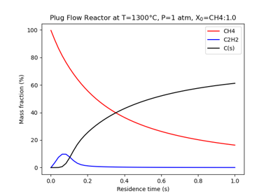
Examples#

Plug Flow Reactor.

`PFRWallProfile` — Prescribed Wall Temperature Profile#

API: bloc.reactors.PFRWallProfile · network: bloc.reactors.PFRWallProfileNet · industrial model: bloc.reactors.TubeFurnace

Physics: The wall temperature is prescribed along the tube axis as \(T_w(x)\) (e.g. the plateau/ramp profile of an electric tube furnace, evaluated by bloc.reactors._wall_T_at). The gas temperature is free and lags the wall through a convective + radiative film. At each after_eval call both components are injected into the energy ODE right-hand side:

\[\dot Q_\mathrm{wall}(x) = \underbrace{h_\mathrm{conv}\,A_\mathrm{int}\,\bigl(T_w(x) - T_g\bigr)}_{\text{forced convection}} \;-\; \underbrace{q_\mathrm{rad}\,A_\mathrm{int}}_{\text{grey-gas radiation}}, \qquad A_\mathrm{int} = \frac{4}{D}\,V\]

The film coefficient comes from a Nusselt correlation for internal pipe flow (bloc.chem.heat_transfer.internal_convection_h(), which selects Baehr-Stephan / Hausen / Churchill-Zajic / \(\mathrm{Nu} = 3.66\) depending on the flow regime and entry length):

\[h_\mathrm{conv} = \frac{\mathrm{Nu}\,k_\mathrm{gas}}{D}, \qquad \mathrm{Re} = \frac{\dot m\,D}{S\,\mu}, \qquad \mathrm{Pr} = \frac{\mu\,c_p}{k_\mathrm{gas}}\]

Gas-to-wall radiation uses the grey-gas approximation with a cylindrical mean-beam-length integral (bloc.chem.heat_transfer.compute_gas2wall_radiative_flux()) — not an optically-thin volumetric law:

\[q_\mathrm{rad} = \left(\frac{2}{3} - f_\mathrm{trans}\right) \sigma\,\bigl(T_g^4 - T_w^4\bigr), \qquad f_\mathrm{trans} = 2\int_0^{\pi/2} e^{-\kappa D \cos\theta}\,\cos^2\theta\,\sin\theta\;\mathrm{d}\theta\]

with \(\kappa\) = kappa_grey; \(\kappa = 0\) disables gas radiation.

SOLVER_MODE = "adaptive" — the network uses net.step() (adaptive step) to resolve the steep temperature gradients near the ramp boundaries.

When to use: Electrically heated tube furnaces with a known, spatially varying wall temperature (plateau + cold legs + ramps). Industrial model: bloc.reactors.TubeFurnace.

`PFRHomogeneousShell` — Homogeneous-Shell Radial Heat Loss#

API: bloc.reactors.PFRHomogeneousShell · network: bloc.reactors.PFRHomogeneousShellNet · industrial model: bloc.reactors.RefractoryReactor

Physics: Thick-walled, heavily insulated vessel where axial wall conduction smears temperature gradients along the shell. The wall is therefore treated as isothermal and the total heat loss is driven by the spatial-mean gas temperature \(\bar T_g\) through a series resistance stack (insulation layers plus external natural convection and radiation):

\[\bar T_g = \frac{1}{L}\int_0^L T_g(x)\,\mathrm{d}x, \qquad \Phi = f_\mathrm{corr}\,\frac{\bar T_g - T_\mathrm{amb}}{R_\mathrm{tot}}\]

\[R_\mathrm{tot} = \sum_i \frac{\ln(r_{i+1}/r_i)}{2\pi k_i L} \;+\; \frac{1}{h_\mathrm{eff}\,S_\mathrm{ext}}, \qquad h_\mathrm{eff} = h_\mathrm{CC} + h_\mathrm{rad}, \qquad h_\mathrm{rad} = 4\,\varepsilon\,\sigma\,T_m^3\]

\(h_\mathrm{CC}\) is the external natural-convection coefficient of a horizontal cylinder (Churchill & Chu, bloc.chem.heat_transfer.compute_hCC_natConv_horizCyl()), \(h_\mathrm{rad}\) the linearised radiative conductance (bloc.chem.heat_transfer.compute_hrad_linearRadiation()), and \(f_\mathrm{corr}\) = heat_loss_corr_factor a lumped multiplier for thermal bridges and other unmodelled loss paths. The stack is solved by bloc.chem.heat_transfer.compute_heat_losses_linear(), which also returns the intermediate layer temperatures (\(\Delta T_i = \Phi,R_i\)) reported as T_wall_ext.

\(\Phi\) is distributed uniformly along the tube through a ct.Wall (area 1 m²) whose flux follows the parcel:

\[q_\mathrm{wall}(t) = -\,\Phi\,\frac{m\,u(t)}{\dot m\,L} \qquad [\mathrm{W/m^2}]\]

Because \(\bar T_g\) depends on the solution and the solution depends on \(\Phi\), the solver uses a Forward-Backward Sweep (FBS):

Adiabatic predictor pass (\(\Phi = 0\)) → \(\bar T_g^{(0)}\).
\(\Phi^{(n)} = \Phi\bigl(\bar T_g^{(n-1)}\bigr)\).
Heated forward pass with \(\Phi^{(n)}\) → \(\bar T_g^{(n)}\).
Iterate until \(\bigl|\Phi^{(n)} - \Phi^{(n-1)}\bigr| \big/ \bigl|\Phi^{(n-1)}\bigr| \<\) CONVERGENCE_TOL (default 1 %), capped at MAX_ITER = 10.

SOLVER_MODE = "fixed_checkpoint" — uniform checkpoints along the axis.

When to use: SPRING reactors (CGR), insulated refractory-lined vessels, any reactor where axial wall conduction prevents local temperature gradients from dominating heat loss. Industrial model: bloc.reactors.RefractoryReactor.

`PFRThinShell` — Thin-Shell Local-Temperature Radial Heat Loss#

API: bloc.reactors.PFRThinShell · network: bloc.reactors.PFRThinShellNet · industrial model: bloc.reactors.QuartzTubeReactor

Physics: Thin-walled reactor (quartz tube, steel tube with negligible axial conduction). The same resistance stack \(R_\mathrm{tot}\) as PFRHomogeneousShell applies, but the driving temperature is the local gas temperature, so the loss is a per-unit-length quantity:

\[q'(z) = -\,f_\mathrm{corr}\,\frac{T_g(z) - T_\mathrm{amb}}{R_\mathrm{tot}\,L} \qquad [\mathrm{W/m}]\]

mapped onto the Cantera Wall convention (W/m² with area 1 m²) by the same \(m,u/\dot m\) scaling as the homogeneous shell. Because \(q'\) depends only on \(T_g(z)\) — never on a solution-wide mean — a single forward pass is sufficient and no FBS iteration is needed. Replacing \(T_g(z)\) by \(\bar T_g\) recovers the homogeneous-shell \(\Phi\), so the two engines share one wall model and differ only in where it is evaluated.

SOLVER_MODE = "fixed_checkpoint" — uniform checkpoints along the axis, no FBS.

When to use: Quartz-tube lab reactors, thin-wall steel tubes, any reactor where axial wall conduction is negligible and the axial gradient is steep enough that a mean-temperature hypothesis would over-predict the loss in the hot zone. Industrial model: bloc.reactors.QuartzTubeReactor.

`PFRGasTemperatureProfile` — Imposed Gas Temperature Profile#

API: bloc.reactors.PFRGasTemperatureProfile · network: bloc.reactors.PFRGasTemperatureProfileNet · procedural equivalent: bloc.reactors.solve_fixed_position_temperature_profile_pfr()

Physics: The gas temperature itself is prescribed along the axis as \(T_\mathrm{prescribed}(x)\) (Dirichlet on the gas). This is the boundary condition the other PFR engines do not cover: PFRWallProfile prescribes the wall temperature and lets the gas lag behind it through a convective + radiative film, whereas here the gas temperature is imposed and the energy equation is switched off — only the kinetics evolve:

\[T_g(x) = T_\mathrm{prescribed}(x) \quad\text{(energy equation disabled)}, \qquad \frac{\mathrm{d}n_k}{\mathrm{d}t} = V\,\dot\omega_k\]

No wall film, no radiation and no resistance stack are involved — the temperature is imposed, not computed from a heat balance. Numerically the closed Lagrangian parcel is marched with march_lagrangian_parcel(..., energy_off=True); the temperature is re-imposed before each checkpoint advance, so the stepwise-constant history converges to the continuous profile as the checkpoint count grows.

SOLVER_MODE = "fixed_checkpoint" — uniform checkpoints along the axis, energy off, no FBS.

When to use: Kinetics validation against a measured in-stream gas temperature (thermocouple trace), or any study where you want predicted species under a known thermal history rather than a predicted temperature.

STONE kind: PFRGasTemperatureProfile. Exceptionally, this numerical engine is registered directly as a STONE kind (no separate industrial-model wrapper): the imposed-gas-temperature march is itself the modelled object.

Key YAML fields: diameter, total_length, T_gas_K, T_ambient_K, entry_leg, exit_leg, entry_zone, plateau_zone, optional T_gas_profile.

Examples#

When to use it

Imposed gas temperature profile (PFRGasTemperatureProfile).

`PSR` — Perfectly Stirred Reactor (base)#

API: bloc.reactors.PSR · industrial model: bloc.reactors.ContinuousMixingReactor

Physics: Well-mixed control volume at constant pressure — the gas is spatially uniform at every instant. In an open stage network Cantera integrates the mole and energy balances with continuous inlet/outlet mass flows until steady state (advance_to_steady_state):

\[\frac{\mathrm{d}n_k}{\mathrm{d}t} = V\,\dot\omega_k + \sum_j \frac{\dot m_j\,Y_{k,j}}{W_k} - \frac{\dot m_\mathrm{out}\,Y_k}{W_k}\]

\[m\,c_p\,\frac{\mathrm{d}T_g}{\mathrm{d}t} = - V \sum_k \bar h_k\,\dot\omega_k + \sum_j \dot m_j \bigl(h_j - h\bigr)\]

where \(j\) runs over the inlet mass-flow controllers, \(Y_{k,j}\) and \(h_j\) are the inlet mass fractions and specific enthalpy, and \(W_k\) is the molar mass of species \(k\). With energy: off the second equation is dropped and \(T_g\) is held fixed.

Network topology:

Stage YAML: OPEN — MFC in, PC/MFC out.
Inner physics: OPEN CSTR (not a closed parcel like the torch).

Common invariants:

ExtensibleIdealGasConstPressureMoleReactor family.
Design residence time t_res_s sizes the volume,

\[V = \frac{\tau\,\dot m}{\rho}\]

applied by Bloc post-build (_post_build_design_volumes). Here \(\tau\) is a design input, not the stage advance_time.

When to use: Continuously-fed well-mixed reactor zones (torch outlet mixing tee, multi-inlet vessel). Industrial model: bloc.reactors.ContinuousMixingReactor.

`InstantaneousMixing` — 0-D HP Mix + Closed Residence-Time Chemistry#

API: bloc.reactors.InstantaneousMixing · network: bloc.reactors.InstantaneousMixingNet · mixer: bloc.reactors.mix_two_streams() · industrial model: bloc.reactors.InstantaneousMixingReactor

Physics: Two inlet streams are combined by constant-enthalpy, constant-pressure algebraic mixing, then a closed parcel integrates ODE chemistry from \(t = 0\) to \(t = \tau\) with no mass exchange during integration.

Step 1 — algebraic HP mix (bloc.reactors.mix_two_streams(), a ct.Quantity sum with constant="HP"):

\[\dot m = \dot m_1 + \dot m_2, \qquad h = \frac{\dot m_1 h_1 + \dot m_2 h_2}{\dot m}, \qquad Y_k = \frac{\dot m_1 Y_{k,1} + \dot m_2 Y_{k,2}}{\dot m}\]

at unchanged \(P\); the mixed temperature follows from the \((h, P, Y_k)\) inversion — no chemistry yet.

Step 2 — closed constant-pressure parcel over the residence time:

\[\frac{\mathrm{d}n_k}{\mathrm{d}t} = V\,\dot\omega_k, \qquad m\,c_p\,\frac{\mathrm{d}T_g}{\mathrm{d}t} = -V \sum_k \bar h_k\,\dot\omega_k, \qquad 0 \le t \le \tau\]

The two steps implement the Da_mix ≫ 1 assumption: turbulent mixing time is much shorter than the chemical relaxation time, so mixing can be treated as instantaneous before chemistry begins.

Network topology:

Stage YAML: OPEN — two inlet MFCs (source reservoirs or upstream outlets), outlet MFC/PC for downstream handoff.
Inner physics: CLOSED parcel (no flux during CVODE integration). MFC rates are used only to identify the two inlet streams and their mass_flow_rate.

When to use: Feedforward one-shot mixing scenarios where the inlets arrive at distinct conditions (temperature, composition) and the mixing timescale is much faster than chemistry. For a continuously-fed CSTR, use bloc.reactors.ContinuousMixingReactor instead.

`TorchInstantaneousHeating` — Instantaneous Enthalpy Jump#

API: bloc.reactors.TorchInstantaneousHeating · network: bloc.reactors.TorchInstantaneousHeatingNet · industrial model: bloc.reactors.PlasmaTorchInstantaneousHeating

Physics: Neither a PFR nor a CSTR. The heating device is collapsed into a single algebraic enthalpy jump at the inlet, followed by an adiabatic constant-pressure kinetic relaxation of a closed parcel. This is the \(\mathrm{Da} \gg 1\) limit for heating: electrical power is deposited on a timescale much shorter than the chemistry it drives.

Step 1 — effective power reaching the gas:

\[P_\mathrm{eff} = \eta_\mathrm{torch}\,\eta_\mathrm{gen}\,P_\mathrm{elec}\]

Step 2 — instantaneous enthalpy increase at constant pressure (gas.HP = gas.h + power_kW * 1e3 / mdot, gas.P in bloc.reactors.TorchInstantaneousHeating.solve_adiabatic()):

\[h^{+} = h^{-} + \frac{P_\mathrm{eff}}{\dot m}, \qquad P^{+} = P^{-}\]

so the specific enthalpy gain of the stream is exactly the specific energy output, \(\Delta h = P_\mathrm{eff}/\dot m = \mathrm{SEO}\). The post-jump temperature is the \((h^{+}, P)\) inversion of the mixture — including whatever dissociation the mechanism predicts at that enthalpy.

Step 3 — adiabatic closed-parcel chemistry over the torch residence time:

\[\frac{\mathrm{d}n_k}{\mathrm{d}t} = V\,\dot\omega_k, \qquad m\,c_p\,\frac{\mathrm{d}T_g}{\mathrm{d}t} = -V \sum_k \bar h_k\,\dot\omega_k, \qquad 0 \le t \le \tau\]

Total enthalpy is conserved from the jump onwards (\(\dot Q_\mathrm{wall} = 0\)): the torch stage carries no wall and no ambient loss. Electrical power is therefore a parameter-backed energy stream rather than a ct.Wall — see the “Energy streams” section of ARCHITECTURE.md.

Specific energy (MJ/kg), exposed as SEI_MJ_kg / SEO_MJ_kg on every torch (bloc.reactors.compute_torch_sei_mj_kg(), bloc.reactors.compute_torch_seo_mj_kg()):

\[\mathrm{SEI} = \frac{P_\mathrm{elec}}{\dot m}, \qquad \mathrm{SEO} = \frac{P_\mathrm{eff}}{\dot m} = \eta_\mathrm{torch}\,\eta_\mathrm{gen}\,\mathrm{SEI}\]

(implemented in kW and kg/s, converted to MJ/kg by \(\times 10^3 / 10^6\)).

Network topology:

Stage YAML: OPEN — inlet MFC, outlet MFC/PC for downstream handoff.
Inner physics: CLOSED parcel. The outlet profile is pre-computed at post-build time by _post_build_design_volumes calling bloc.reactors.TorchInstantaneousHeating.solve_adiabatic(); the stage network only validates and exposes it.

When to use: Any heating device — plasma torch, arc heater, resistive pre-heater — whose energy deposition is fast compared with the chemistry, and where a spatially resolved arc model is not needed. Industrial model: bloc.reactors.PlasmaTorchInstantaneousHeating.

Industrial Models#

Industrial models are thin concrete subclasses of the engine classes. They add domain-specific parameter names, default values, KPI extractors, and documentation. They do not change the underlying physics — with the single exception of bloc.reactors.SootRadiatingTubeFurnace, which overrides the radiation closure (documented below).

`TubeFurnace` ← `PFRWallProfile`#

API: bloc.reactors.TubeFurnace · network: bloc.reactors.PFRWallProfileNet · wall profile: bloc.reactors._wall_T_at

Electric tube furnace with a spatially varying internal wall temperature (plateau + entry/exit ramps + unheated cold legs). The equations are those of bloc.reactors.PFRWallProfile: forced convection plus grey-gas radiation against the prescribed \(T_w(x)\).

STONE kind: TubeFurnace

Key YAML fields: diameter, total_length, T_wall_K, T_ambient_K, entry_leg, exit_leg, entry_zone, plateau_zone, kappa_grey, mass_flow_rate.

KPI function: bloc.reactors.compute_tube_furnace_kpis() (bloc.reactors:compute_tube_furnace_kpis)

Examples#

Flow effects on axial temperature profiles.

ctwrap interface

Tube furnace – N₂ temperature profiles vs. Mei et al. (2019).

`SootRadiatingTubeFurnace` ← `TubeFurnace`#

API: bloc.reactors.SootRadiatingTubeFurnace · network: bloc.reactors.PFRWallProfileNet

Same convection and mean-beam-length radiation as bloc.reactors.TubeFurnace, but the grey-gas absorption coefficient is augmented by the local soot loading instead of staying at the fixed kappa_grey, using the Planck-mean grey-gas correlation (Rodrigues):

\[\kappa_\mathrm{eff} = \kappa_\mathrm{grey} + 3.83\,\frac{C_0}{C_2}\,f_v\,T_g, \qquad f_v = \frac{Y_\mathrm{soot}\,\rho_\mathrm{gas}}{\rho_\mathrm{soot}}\]

with \(C_0 = 6\pi E(m)\) the soot optical constant (\(E(m) \approx 0.260\)), \(C_2 = hc/k_B \approx 0.014388\) m·K the second radiation constant, and \(Y_\mathrm{soot}\) the summed solid-carbon mass fraction above the mechanism’s n_C_min threshold. kappa_grey therefore carries the clean-gas baseline, and \(\kappa_\mathrm{eff}\) feeds the same \(q_\mathrm{rad}\) expression as the base class.

STONE kind: SootRadiatingTubeFurnace

Key YAML fields: those of TubeFurnace, plus soot_density (default 1800 kg/m³) and optional n_C_min (auto-resolved from the mechanism when omitted).

`RefractoryReactor` ← `PFRHomogeneousShell`#

API: bloc.reactors.RefractoryReactor · network: bloc.reactors.PFRHomogeneousShellNet

Insulated refractory-lined growth reactor (CGR in SPRING). Uses the homogeneous-shell heat-loss model with Forward-Backward Sweep — the \(\bar T_g \rightarrow \Phi \rightarrow \bar T_g\) iteration documented under bloc.reactors.PFRHomogeneousShell.

STONE kind: RefractoryReactor (YAML node id CGR is a user convention)

Key YAML fields: length, diameter, mass_flow_rate, eps_wall, T_wall_hyp, T_amb, insulation, adiabatic, heat_loss_corr_factor.

Examples#

Benchmark three PFR approaches on the same adiabatic case.

When to use this script

Minimal runnable RefractoryReactor / PFRHomogeneousShellNet example.

`QuartzTubeReactor` ← `PFRThinShell`#

API: bloc.reactors.QuartzTubeReactor · network: bloc.reactors.PFRThinShellNet

Quartz-tube or thin-wall lab reactor. Uses the thin-shell local-\(T\) heat-loss model — single forward pass, \(q'(z) \propto T_g(z) - T_\mathrm{amb}\).

STONE kind: QuartzTubeReactor

Key YAML fields: same as RefractoryReactor.

`ContinuousMixingReactor` ← `PSR`#

API: bloc.reactors.ContinuousMixingReactor

Multi-inlet well-mixed open CSTR (TMR in SPRING). Accepts multiple inlet: ports and solves the open mole/energy balances of bloc.reactors.PSR. Volume is sized by Bloc post-build using \(V = \tau,\dot m / \rho\).

STONE kind: ContinuousMixingReactor (YAML node id TMR is a user convention)

Key YAML fields: t_res_s, temperature, pressure, composition.

Mixing model: Da_mix ≫ 1 assumed. Inlet streams are stirred by Cantera’s MFC topology inside the open CSTR until advance_to_steady_state. This is appropriate when the mixing and chemistry occur simultaneously in a continuously-fed vessel.

`InstantaneousMixingReactor` ← `InstantaneousMixing` ← `PSR`#

API: bloc.reactors.InstantaneousMixingReactor · network: bloc.reactors.InstantaneousMixingNet

Two-inlet reactor that combines algebraic HP mixing with closed-parcel chemistry — the two-step formulation of bloc.reactors.InstantaneousMixing.

STONE kind: InstantaneousMixingReactor

Key YAML fields: t_res_s, temperature, pressure, composition.

Requires exactly two inlet MassFlowController connections. Bloc post-build (_post_build_design_volumes) gathers both inlet states and mass flow rates, calls bloc.reactors.InstantaneousMixing.solve_premixed(), and writes the outlet back to reactor.phase + syncState().

When to choose over ContinuousMixingReactor:

Criterion	`ContinuousMixingReactor`	`InstantaneousMixingReactor`
Feed mode	Continuously fed	One-shot feedforward
Chemistry	CSTR (open, steady-state)	Closed parcel (no MFC flux)
Mixing	In-vessel MFC stirring	Algebraic HP mix before chemistry
Da_mix assumption	Implicit (well-mixed vessel)	Explicit (Da_mix ≫ 1)
`t_res_s` role	Sizes volume via \(V = \tau\dot m/\rho\)	CVODE integration horizon
`is_psr` meta	True	False

`InstantaneousQuenchReactor` ← `InstantaneousMixing` ← `PSR`#

API: bloc.reactors.InstantaneousQuenchReactor · network: bloc.reactors.InstantaneousMixingNet

Same closed-τ mechanics as InstantaneousMixingReactor, but with the unknown on the other side: given a single real hot-gas inlet and a quench gas of known temperature/composition (T_quench_C, X_quench — node properties, not a second inlet connection), the quench mass flow is solved for via bloc.reactors.find_quench_flow() to hit target_temperature_C, then mixed with bloc.reactors.mix_two_streams() and integrated for t_res_s exactly like InstantaneousMixingReactor.

STONE kind: InstantaneousQuenchReactor

Key YAML fields: t_res_s, T_quench_C, X_quench (a composition string/dict, or the id of another node in the network whose composition should be reused — e.g. the hot inlet’s own id), target_temperature_C.

Referencing a node id reuses only that node’s gas-phase fraction: solid-carbon species (soot/PAH bins) are filtered out via bloc.chem.solid_carbon_threshold.resolve_n_c_min() and the remainder renormalized to 1 — i.e. it assumes the solid fraction has already been filtered out of that stream before it becomes quench media, not that the referenced node’s raw, as-solved composition is reused verbatim. This can make the resulting quench-gas HHV noticeably higher per kg than the referenced node’s own overall HHV, since removing a low-HHV-per-kg solid fraction and renormalizing concentrates the remaining light species.

Requires exactly one inlet MassFlowController connection (the hot gas). Bloc post-build (_post_build_design_volumes) resolves that inlet, solves for the quench flow, calls bloc.reactors.InstantaneousMixing.solve_premixed(), and writes the outlet back to reactor.phase + syncState() — same as InstantaneousMixingReactor.

`PlasmaTorchInstantaneousHeating` ← `TorchInstantaneousHeating`#

API: bloc.reactors.PlasmaTorchInstantaneousHeating · network: bloc.reactors.TorchInstantaneousHeatingNet

Plasma torch modelled as an instantaneous enthalpy injection followed by chemical equilibration — the three-step formulation of bloc.reactors.TorchInstantaneousHeating, with \(P_\mathrm{eff} = \eta_\mathrm{torch},\eta_\mathrm{gen},P_\mathrm{elec}\) and \(\Delta h = P_\mathrm{eff}/\dot m\). Not a PFR. The InstantaneousHeating suffix reserves the namespace for future torch models with different heating physics (arc-discharge, spatially resolved, or multi-temperature).

STONE kind: PlasmaTorchInstantaneousHeating

Key YAML fields: electric_power_kW, torch_eff, gen_eff, t_res_s, temperature, pressure, composition.

Specific energy (MJ/kg). Every torch (this class and its subclasses) exposes SEI_MJ_kg / SEO_MJ_kg on bloc.reactors.TorchInstantaneousHeating, populated by _post_build_design_volumes from electric_power_kW, effective_power_kW (\(= P_\mathrm{elec},\eta_\mathrm{torch},\eta_\mathrm{gen}\)) and the resolved mass_flow_rate:

SEI (Specific Energy Input) = electric_power_kW·1e3 / mdot / 1e6
SEO (Specific Energy Output) = effective_power_kW·1e3 / mdot / 1e6

They are shown in the Torch pane (bloc/boulder_plugins/torch_pane.py).

`ThreeSegmentsReactor` — composite tube → mix → tube chain#

API: bloc.reactors.ThreeSegmentsReactor · network: bloc.reactors.ThreeSegmentsReactorNet

Composite unit operation: \(N\) bloc.reactors.RefractoryReactor segments in series with \(M = N - 1\) bloc.reactors.InstantaneousMixing injection points between them (the SPRING CGR with staged injection). The outer reactor is a placeholder — it holds the outlet stream point and metadata; all physics live in the network, which composes the per-segment FBS solve with the algebraic HP mixers:

\[\text{segment } i:\quad \bigl(T_\mathrm{in}, P, Y_k\bigr)_i \;\xrightarrow[\ \text{FBS}\ ]{\ \Phi_i\ }\; \bigl(T_\mathrm{out}, P, Y_k\bigr)_i\]

\[\text{injection } i:\quad h^\mathrm{in}_{i+1} = \frac{\dot m_i\,h^\mathrm{out}_i + \dot m_{\mathrm{inj},i}\,h_{\mathrm{inj},i}} {\dot m_i + \dot m_{\mathrm{inj},i}}, \qquad \dot m_{i+1} = \dot m_i + \dot m_{\mathrm{inj},i}\]

Each segment carries its own resistance stack and converges its own \(\Phi_i\); the composite reports the aggregates

\[\Phi_\mathrm{tot} = \sum_i \Phi_i, \qquad \tau_\mathrm{tot} = \sum_i \tau_i, \qquad L_\mathrm{tot} = \sum_i L_i\]

and a single spatial profile obtained by concatenating the segment profiles with an axial offset \(x_i = \sum_{j\<i} L_j\).

STONE kind: ThreeSegmentsReactor

Key YAML fields: the per-segment RefractoryReactor properties plus the injection descriptors; the unfolder expands the composite node into segment and mixer nodes at normalize_config time.

Supplier equipment models#

Named products from suppliers, under bloc.reactors.models. They reuse a generic engine and add a nameplate operating envelope (enforced at build time) plus datasheet-specific KPIs.

`PBR100PlasmaTorch` ← `PlasmaTorchInstantaneousHeating`#

API: bloc.reactors.PBR100PlasmaTorch · network: bloc.reactors.TorchInstantaneousHeatingNet

The PBR 100 arc-heated plasma source. Same instantaneous-heating physics and equations as bloc.reactors.PlasmaTorchInstantaneousHeating; adds:

Envelope validation (raises at build time when outside range): performance 50–100 kW (electric_power_kW, schema-enforced); CH4 5–20 kg/h; H2 20–100 slm; N2 100–350 slm (throughput checked from the resolved inlet in _post_build_design_volumes).
Specific energy (MJ/kg): SEI/SEO are inherited from the base torch class (see PlasmaTorchInstantaneousHeating above) and shown in the Torch pane.

STONE kind: PBR100PlasmaTorch

Key YAML fields: electric_power_kW (50–100), torch_eff, gen_eff, t_res_s, temperature, pressure, composition.

Kind rename map#

The table below maps the legacy Design* YAML kinds to the current names. Legacy kinds are no longer registered — new and existing YAML files should use the current names.

Legacy kind	Current kind	Engine base
`DesignTubeFurnace`	`TubeFurnace`	`PFRWallProfile`
`DesignPFR`	`RefractoryReactor`	`PFRHomogeneousShell`
`DesignPFRThinShell`	`QuartzTubeReactor`	`PFRThinShell`
`DesignPSR`	`ContinuousMixingReactor`	`PSR`
`DesignTorchInstantaneousHeating`	`PlasmaTorchInstantaneousHeating`	`TorchInstantaneousHeating`

`PFRNetwork` — Unified network driver#

bloc.reactors.PFRNetwork is the generic driver for all bloc.reactors.PFR subclasses. It dispatches on SOLVER_MODE:

"adaptive" — uses Cantera’s net.step() for each spatial checkpoint. Used by PFRWallProfile / TubeFurnace.
"fixed_checkpoint" — advances to each checkpoint with net.advance(t_check). May iterate (FBS) when PFRHomogeneousShell is used. Single-pass for PFRThinShell.

All PFR engines set NETWORK_CLASS = PFRNetwork; the registered industrial models override it with the specialised network listed in their section above and in the registration table of ARCHITECTURE.md.

Reactor Types#

Architecture overview#

Notation#

Why not Cantera’s FlowReactor?#

Numerical engines#

PFR — Plug Flow Reactor (base)#

Examples#

PFRWallProfile — Prescribed Wall Temperature Profile#

PFRHomogeneousShell — Homogeneous-Shell Radial Heat Loss#

PFRThinShell — Thin-Shell Local-Temperature Radial Heat Loss#

PFRGasTemperatureProfile — Imposed Gas Temperature Profile#

Examples#

PSR — Perfectly Stirred Reactor (base)#

InstantaneousMixing — 0-D HP Mix + Closed Residence-Time Chemistry#

TorchInstantaneousHeating — Instantaneous Enthalpy Jump#

Industrial Models#

TubeFurnace ← PFRWallProfile#

Examples#

SootRadiatingTubeFurnace ← TubeFurnace#

RefractoryReactor ← PFRHomogeneousShell#

Examples#

QuartzTubeReactor ← PFRThinShell#

ContinuousMixingReactor ← PSR#

InstantaneousMixingReactor ← InstantaneousMixing ← PSR#

InstantaneousQuenchReactor ← InstantaneousMixing ← PSR#

PlasmaTorchInstantaneousHeating ← TorchInstantaneousHeating#

ThreeSegmentsReactor — composite tube → mix → tube chain#

Supplier equipment models#

PBR100PlasmaTorch ← PlasmaTorchInstantaneousHeating#

Kind rename map#

PFRNetwork — Unified network driver#

Why not Cantera’s `FlowReactor`?#

`PFR` — Plug Flow Reactor (base)#

`PFRWallProfile` — Prescribed Wall Temperature Profile#

`PFRHomogeneousShell` — Homogeneous-Shell Radial Heat Loss#

`PFRThinShell` — Thin-Shell Local-Temperature Radial Heat Loss#

`PFRGasTemperatureProfile` — Imposed Gas Temperature Profile#

`PSR` — Perfectly Stirred Reactor (base)#

`InstantaneousMixing` — 0-D HP Mix + Closed Residence-Time Chemistry#

`TorchInstantaneousHeating` — Instantaneous Enthalpy Jump#

`TubeFurnace` ← `PFRWallProfile`#

`SootRadiatingTubeFurnace` ← `TubeFurnace`#

`RefractoryReactor` ← `PFRHomogeneousShell`#

`QuartzTubeReactor` ← `PFRThinShell`#

`ContinuousMixingReactor` ← `PSR`#

`InstantaneousMixingReactor` ← `InstantaneousMixing` ← `PSR`#

`InstantaneousQuenchReactor` ← `InstantaneousMixing` ← `PSR`#

`PlasmaTorchInstantaneousHeating` ← `TorchInstantaneousHeating`#

`ThreeSegmentsReactor` — composite tube → mix → tube chain#

`PBR100PlasmaTorch` ← `PlasmaTorchInstantaneousHeating`#

`PFRNetwork` — Unified network driver#