bloc.reactors#

Custom Cantera reactor extensions and solvers.

Submodules#

Attributes#

`Pr_air_20C`
`alpha_air_20C`
`conductivity_air_20C`
`nu_air_20C`
`sigma_SB`

Classes#

`DesignIdealGasConstPressureMoleReactor`	Design-oriented constant-pressure mole reactor with helper APIs.
`ThreeSegmentsReactor`	Placeholder reactor for the CGR composite unit operation.
`ThreeSegmentsReactorNet`	Composite stage network for the CGR unit operation.
`PBR100PlasmaTorch`	PBR 100 — arc-heated plasma source (instantaneous-heating variant).
`PFRGasTemperatureProfileNet`	Stage network driving a `PFRGasTemperatureProfile`.
`PFRHomogeneousShellNet`	ReactorNet subclass implementing Forward-Backward Sweep for a PFR stage.
`PFRThinShellNet`	Single-pass PFR network for the thin-shell hypothesis.
`QuartzTubeReactor`	Industrial quartz-tube / lab-tube reactor.
`RefractoryReactor`	Industrial Carbon Growth Reactor (CGR) / refractory-lined vessel.
`PFR`	Plug Flow Reactor (PFR) engine — closed Lagrangian parcel march.
`PFRGasTemperatureProfile`	PFR engine with a prescribed GAS temperature profile T_gas(x).
`PFRHomogeneousShell`	PFR engine with homogeneous-shell radial heat loss.
`PFRNetwork`	Unified network driver for any `PFR` subclass.
`PFRThinShell`	PFR engine with thin-shell local-temperature radial heat loss.
`PFRWallProfile`	PFR engine with a prescribed wall-temperature profile.
`PSR`	Perfectly Stirred Reactor (PSR) engine — well-mixed, constant-pressure.
`CarbonBlackIdealGasConstPressureReactor`	IdealGasConstPressureReactor with additional features for carbon quality calculations.
`CarbonBlackIdealGasMoleReactor`	IdealGasMoleReactor with additional features for carbon quality calculations.
`CarbonBlackIdealGasReactor`	IdealGasReactor with additional features for carbon quality calculations.
`ContinuousMixingReactor`	Industrial Torch Mixing Reactor (TMR) / multi-inlet well-mixed vessel.
`InstantaneousMixing`	Engine: instantaneous HP mix of two inlet streams + closed-τ chemistry.
`InstantaneousMixingNet`	ReactorNet subclass for instantaneous-mix + closed-τ chemistry.
`InstantaneousMixingReactor`	Industrial model: instantaneous mix + closed chemical residence time.
`PlasmaTorchInstantaneousHeating`	Industrial Plasma Torch model — instantaneous-heating variant.
`TorchInstantaneousHeating`	Torch physics engine with instantaneous enthalpy jump (plasma / simplified).
`TorchInstantaneousHeatingNet`	ReactorNet subclass implementing torch adiabatic integration.
`PFRWallProfileNet`	Stage network driving a `TubeFurnace` through a prescribed wall profile.
`SootRadiatingTubeFurnace`	Tube furnace with soot-augmented grey-gas radiation.
`TubeFurnace`	Industrial Tube Furnace model.

Functions#

`compute_gas2wall_radiative_flux`(T_g, T_w, kappa_grey, D)	Radiative flux from a participating gas to the tube wall in W/m2.
`compute_hCC_natConv_horizCyl`(diameter, length, ...[, ...])	Natural convection coefficient at the external wall of a horizontal cylinder.
`compute_hCC_natConv_vertCyl`(diameter, length, ...[, ...])	Natural convection coefficient at the external wall of a vertical cylinder.
`compute_heat_losses_linear`(Tr_C, Tamb_C, R_list)	Solve heat transfer through a series thermal resistance stack.
`compute_hrad_linearRadiation`(eps, Tmoy)	Linearized radiative conductance for small temperature differences.
`internal_convection_h`(diameter, mass_flow_rate, gas[, ...])	Compute internal forced convection coefficient for gas in a circular tube.
`thermal_resistance_CC`(h_CC, S)	Thermal resistance of a conducto-convective heat transfer surface.
`thermal_resistance_radial_conduction`(diameter, length, ...)	Thermal resistance for radial conduction in cylindrical geometry.
`find_temperature_from_enthalpy`(h_mass, X, P_bar, mechanism)	Return the temperature in °C for a given enthalpy in J/kg and for a given gas composition and pressure.
`switch_mechanism`(gas, new_mechanism[, htol, Xtol, verbose])	Switch the mechanism of a gas object.
`get_solid_carbon_mass_fraction`(gas[, solid_sp, n_C_min])	Return the mass fraction of solid carbon species in the gas object.
`build_closed_carrier_net`(reactor, T, P, X, volume, *)	Build a fresh CLOSED carrier reactor (no flow devices) and a bare ReactorNet.
`copy_state`(src_phase, dst_reactor)	Copy outlet TPX from src_phase back onto the stage dst_reactor.
`march_lagrangian_parcel`(reactor, T_in, P_in, X_in, *, ...)	Single forward pass of a CLOSED Lagrangian parcel from inlet to outlet.
`find_2nd_inj_mass_flow_rate`(gas_torch, qm_torch, ...)	Find the mass flow rate (in kg/s) of the second injection to reach the desired temperature in the reactor.
`find_2nd_inj_mfr_Tin`(gas_torch, qm_torch, gas_2nd_inj, ...)	Find the mass flow rate (in kg/s) of the 2nd injection to reach the desired temperature at the reactor entrance.
`find_2nd_inj_mfr_Tout`(gas_torch, qm_torch, ...[, ...])	Find the mass flow rate (in kg/s) of the second injection to reach the desired specific enthalpy at the reactor output.
`find_2nd_inj_mfr_Tout_generalized`(gas_torch, qm_torch, ...)	Find the mass flow rate (in kg/s) of the second injection to reach the desired specific enthalpy
`find_quench_flow`(qm_reac, gas_reac, X_quench, ...[, ...])	Compute the required quench mass flow for a desired mixed outlet temperature.
`is_pfr_profile_kind`(kind)	Return True when kind is a registered STONE kind for any PFR/CGR profile reactor.
`residence_states_to_series`(states)	Serialize a closed CSTR residence-time profile for the Plots tab.
`states_to_series`(states[, fbs_convergence])	Serialize a spatial `SolutionArray` profile to a JSON-compatible dict.
`compute_reactor_dimensions_with_form_factor`(qm_in, ...)
`compute_reactor_length`(qm_in, S_in, states)	qm_in = v * S_in * density <=> v = qm_in / (S_in*density).
`compute_recovered_power`(qm_torch, T_torch_input_C, ...)	Compute the power recovered from the preheating of the torch and the second injection.
`compute_residual_heat`(P_recovered, gas, qm_tot, T_amb_C)	Compute residual heat after recovery in the exchanger.
`get_carbon_yield`(gas[, n_C_min])	Compute carbon yield (solid C mass / total C mass in feed).
`get_H2_yield`(states)	Compute the H2 yield of the process from the states object.
`get_reactor_mass`(L_reactor, d_reactor, e_insul_layers, ...)	Compute the mass of the reactor based on its dimensions and the insulation layers.
`mix_two_streams`(gas_1, qm_1, gas_2, qm_2)	Mix two streams of gases and return the resulting cantera.Quantity object.
`solve_adiabatic_reactor`(qm_kgs, P_in_kW, t_res, X0, ...)	Solve the kinetics in an adiabatic isobaric reactor at P_bar (bar) for a residence time t_res (s).
`solve_fixed_position_temperature_profile_pfr`(qm_kgs, ...)	Solve kinetics in a PFR with a prescribed temperature profile T(x).
`solve_fixed_time_enthalpy_profile_pfr`(...[, dt, ...])	Solve kinetics in a PFR with a prescribed specific-enthalpy profile h(t).
`solve_fixed_time_heat_flux_pfr`(inlet_composition, ...)	Solve kinetics in a PFR heated by a temperature-difference-driven flux.
`solve_fixed_time_temperature_profile_pfr`(...[, dt, ...])	Solve kinetics in a PFR with a prescribed temperature profile T(t).
`solve_isothermal_reactor`(qm_kgs, T_reactor_C, t_res, ...)	Solve the kinetics in an isothermal isobaric reactor at T_reactor_C (°C) and P_bar (bar) for a residence time t_res (s).
`is_psr_mixing_kind`(kind)	Return True when kind is a registered STONE kind for any PSR-family mixer.
`compute_torch_sei_mj_kg`(electric_power_kW, mdot_kg_s)	Specific Energy Input [MJ/kg] = electrical input per kg of feed.
`compute_torch_seo_mj_kg`(effective_power_kW, mdot_kg_s)	Specific Energy Output [MJ/kg] = thermal power to gas per kg of feed.
`is_torch_reactor_kind`(kind)	Return True when kind is a registered STONE kind for any torch.
`compute_tube_furnace_kpis`(sim)	Compute tube-furnace engineering KPIs from a solved STONE Simulation.

Package Contents#

bloc.reactors.Pr_air_20C = 0.707#

bloc.reactors.alpha_air_20C = 2.25e-05#

bloc.reactors.compute_gas2wall_radiative_flux(T_g, T_w, kappa_grey, D)#

Radiative flux from a participating gas to the tube wall in W/m2.

Uses the grey gas approximation with cylindrical geometry (mean beam length approximation via spherical integral).

Assumptions:

Temperature and composition are uniform in the cross-section.
Grey body gas with absorption coefficient kappa_grey.
Walls are black (covered by soot); no wall reflection.

\[ \begin{align}\begin{aligned}f_{\mathrm{trans}} = 2 \int_0^{\pi/2} e^{-\kappa D \cos\theta} \cos^2\theta \sin\theta \, d\theta\\q_{\mathrm{rad}} = \left(\frac{2}{3} - f_{\mathrm{trans}}\right) \sigma_{\mathrm{SB}} (T_g^4 - T_w^4)\end{aligned}\end{align} \]

Positive q_rad means net heat transfer from gas to wall.

Parameters:

T_g (float) – Gas temperature in K.
T_w (float) – Wall temperature in K.
kappa_grey (float) – Grey gas absorption coefficient in 1/m. Use kappa_grey = 0 to disable gas radiation.
D (float) – Tube inner diameter in m.

Returns:

q_rad (float) – Net radiative heat flux from gas to wall in W/m2.
f_trans (float) – Transmittance factor (dimensionless).

bloc.reactors.compute_hCC_natConv_horizCyl(diameter, length, T_wall_C, T_amb_C, conductivity=conductivity_air_20C, nu=nu_air_20C, alpha=alpha_air_20C, Pr=Pr_air_20C)#

Natural convection coefficient at the external wall of a horizontal cylinder.

Uses Churchill & Chu (1975) correlation.

\[ \begin{align}\begin{aligned}\mathrm{Ra}_D = \frac{g \beta (T_{\mathrm{wall}} - T_{\mathrm{amb}}) D^3}{\nu \alpha}\\\mathrm{Nu}_D = \left(0.6 + \frac{0.387 \mathrm{Ra}_D^{1/6}} {(1 + (0.559/\mathrm{Pr})^{9/16})^{8/27}}\right)^2, \quad h = \frac{\mathrm{Nu}_D \, k}{D}\end{aligned}\end{align} \]

Parameters:

diameter (float) – Outer diameter in m.
length (float) – Cylinder length in m (unused in this correlation, kept for API consistency).
T_wall_C (float) – Wall temperature in deg C.
T_amb_C (float) – Ambient temperature in deg C.
conductivity (float, optional) – Fluid thermal conductivity in W/m/K. Defaults to air at 20 deg C.
nu (float, optional) – Kinematic viscosity in m2/s. Defaults to air at 20 deg C.
alpha (float, optional) – Thermal diffusivity in m2/s. Defaults to air at 20 deg C.
Pr (float, optional) – Prandtl number. Defaults to air at 20 deg C.

Returns:

Convective heat transfer coefficient h in W/m2/K.

Return type:

float

bloc.reactors.compute_hCC_natConv_vertCyl(diameter, length, T_wall_C, T_amb_C, conductivity=conductivity_air_20C, nu=nu_air_20C, alpha=alpha_air_20C, Pr=Pr_air_20C)#

Natural convection coefficient at the external wall of a vertical cylinder.

Correlation from Taine / Lefevre (1956).

Warning

Valid for laminar flow only; gives low h values.

\[ \begin{align}\begin{aligned}\mathrm{Ra}_L = \frac{g \beta (T_{\mathrm{wall}} - T_{\mathrm{amb}}) L^3}{\nu \alpha}\\\mathrm{Nu} = \frac{4}{3} \left(\frac{7 \mathrm{Ra}_L \mathrm{Pr}}{100 + 105 \mathrm{Pr}}\right)^{1/4} + 0.1143 \frac{272 + 315 \mathrm{Pr}}{64 + 63 \mathrm{Pr}} \frac{L}{D}, \quad h = \frac{\mathrm{Nu} \, k}{L}\end{aligned}\end{align} \]

Parameters:

diameter (float) – Outer diameter in m.
length (float) – Cylinder length in m.
T_wall_C (float) – Wall temperature in deg C.
T_amb_C (float) – Ambient temperature in deg C.
conductivity (float, optional) – Fluid thermal conductivity in W/m/K. Defaults to air at 20 deg C.
nu (float, optional) – Kinematic viscosity in m2/s. Defaults to air at 20 deg C.
alpha (float, optional) – Thermal diffusivity in m2/s. Defaults to air at 20 deg C.
Pr (float, optional) – Prandtl number. Defaults to air at 20 deg C.

Returns:

Convective heat transfer coefficient h in W/m2/K.

Return type:

float

bloc.reactors.compute_heat_losses_linear(Tr_C, Tamb_C, R_list)#

Solve heat transfer through a series thermal resistance stack.

\[R_{\mathrm{tot}} = \sum_i R_i, \quad \Phi = \frac{T_{\mathrm{reac}} - T_{\mathrm{amb}}}{R_{\mathrm{tot}}}, \quad \Delta T_i = \Phi \, R_i\]

Parameters:

Tr_C (float) – Temperature inside the reactor in deg C.
Tamb_C (float) – Ambient temperature in deg C.
R_list (list of float) – Thermal resistances in K/W, ordered from reactor interior to ambient.

Returns:

{"Phi": float, "T_reac": float, "T_wall_ext": float, "T_amb": float, ...} where Phi is heat loss in W.

Return type:

dict

bloc.reactors.compute_hrad_linearRadiation(eps, Tmoy)#

Linearized radiative conductance for small temperature differences.

\[h_{\mathrm{rad}} = \varepsilon \sigma_{\mathrm{SB}} \, 4 T_{\mathrm{moy}}^3\]

Parameters:

eps (float) – Emissivity, dimensionless.
Tmoy (float) – Mean temperature in K.

Returns:

Linearized radiative heat transfer coefficient in W/m2/K.

Return type:

float

bloc.reactors.conductivity_air_20C = 0.0263#

bloc.reactors.internal_convection_h(diameter, mass_flow_rate, gas, x_position=None)#

Compute internal forced convection coefficient for gas in a circular tube.

Delegates to ht.conv_internal.Nu_conv_internal() [CalebBell_ht] which dynamically selects the most accurate applicable correlation:

Laminar developing flow (Re < 2300, x_position provided): Baehr-Stephan laminar thermal/velocity entry.
Laminar fully-developed (Re < 2300, no x_position): Constant wall temperature, Nu = 3.66.
Turbulent with entry effects (Re > 4000, x_position provided): Hausen.
Turbulent general (Re > 4000): Churchill-Zajic.
Turbulent, low Prandtl (Pr < 0.03): Martinelli.

Transport properties (viscosity, thermal conductivity, heat capacity) are read from the Cantera Solution object at the current state. The gas mechanism must define a transport model (e.g. Mix or Multi); mechanisms with transport_model == 'none' are not supported.

Parameters:

diameter (float) – Tube inner diameter in m.
mass_flow_rate (float) – Mass flow rate through the tube in kg/s.
gas (cantera.Solution) – Gas object at the current thermodynamic state (must have transport).
x_position (float or None, optional) – Distance from the tube inlet in m. When provided, entry-length correlations are used; otherwise fully-developed flow is assumed.

Returns:

Convective heat transfer coefficient h in W/m2/K.

Return type:

float

Raises:

ValueError – If gas.transport_model == 'none' (mechanism has no transport data).

See also

ht.conv_internal.Nu_conv_internal: Underlying correlation selector from the ht library.

Notes

For CH4 pyrolysis conditions (10 SLM, D = 100 mm), Re ~ 130–250 across the full temperature range (25–1600 deg C), so fully-developed laminar flow applies and Nu = 3.66. Radiation dominates at high temperatures.

bloc.reactors.nu_air_20C = 1.589e-05#

bloc.reactors.sigma_SB = 5.67e-08#

bloc.reactors.thermal_resistance_CC(h_CC, S)#

Thermal resistance of a conducto-convective heat transfer surface.

\[R = \frac{1}{h_{\mathrm{CC}} \, S}\]

Parameters:

h_CC (float) – Heat transfer coefficient in W/m2/K.
S (float) – Surface area in m2.

Returns:

Thermal resistance in K/W.

Return type:

float

bloc.reactors.thermal_resistance_radial_conduction(diameter, length, conductivity, e_insulation)#

Thermal resistance for radial conduction in cylindrical geometry.

\[R = \frac{\ln(r_2/r_1)}{2\pi k L}, \quad r_1 = D/2, \quad r_2 = D/2 + e_{\mathrm{insulation}}\]

Parameters:

diameter (float) – Inner diameter in m.
length (float) – Cylinder length in m.
conductivity (float) – Thermal conductivity of insulation in W/m/K.
e_insulation (float) – Insulation thickness in m.

Returns:

Thermal resistance in K/W.

Return type:

float

bloc.reactors.find_temperature_from_enthalpy(h_mass, X, P_bar, mechanism)#

Return the temperature in °C for a given enthalpy in J/kg and for a given gas composition and pressure.

Parameters:

h_mass (-) – Specific enthalpy target in J/kg
X (-) – Composition of the gas in mole fraction
P_bar (-) – Pressure in bar
mechanism (-) – Path to the mechanism file

bloc.reactors.switch_mechanism(gas, new_mechanism, htol=0.0001, Xtol=0.0001, verbose=False)#

Switch the mechanism of a gas object.

Useful to switch from plasma to reactor simulation for instance. As some species may not be present in the new mechanism, we compute the adjust the temperature of the new gas object to match the enthalpy of the old gas object, so that energy is conserved. Still, if the chemical enthalpy variation exceed htol, an error is raised. Similarly, if the mole fraction variation exceed Xtol, a error is raised.

Parameters:

gas (ct.Solution) – Gas object
new_mechanism (str) – Path to the new mechanism file
htol (float) – Tolerance for the chemical enthalpy variation between the two mechanisms. Default is 1e-4.
Xtol (float) – Tolerance for the mole fraction variation between the two mechanisms. Default is 1e-4.
verbose (bool) – If True, print information about the process. Default is False.

Returns:

gas_new – Gas object with the new mechanism

Return type:

ct.Solution

bloc.reactors.get_solid_carbon_mass_fraction(gas, solid_sp=['C(s)', 'C(soot)', 'CSOLID'], n_C_min=300)#

Return the mass fraction of solid carbon species in the gas object.

Solid species are identified by their name or by the number of carbon atoms, through get_solid_carbon_species().

Parameters:

gas (cantera.Solution) – The gas object containing gaseous species and soot.
solid_sp (list of str, optional) – List of solid species to consider. Default is [“C(s)”, “C(soot)”, “CSOLID”].
n_C_min (int, optional) – Minimum number of carbon atoms to consider a species as solid. Default is 300. This is used as a second filter to identify solid carbon species. A specie is considered solid if it satisfies one criterium (s in solid_sp) OR the other (n_C >= n_C_min).

Returns:

The mass fraction of solid carbon species in the gas object.

Return type:

float

class bloc.reactors.DesignIdealGasConstPressureMoleReactor(gas, *args, **kwargs)#

Bases: cantera.ExtensibleIdealGasConstPressureMoleReactor

Design-oriented constant-pressure mole reactor with helper APIs.

Inherits from ExtensibleIdealGasConstPressureMoleReactor so that subclasses can intercept Cantera’s ODE callbacks without modifying C++ code.

The key hook used here is before_update_state(): CVODE calls updateState(y) before its very first eval, at which point y is still writable. By storing a pending initial condition in _pending_init and writing it into y on the first call, any subclass can override CVODE’s starting point — even though m_state (the C++ snapshot taken at construction) cannot be changed from Python.

Parameters:: gas – Cantera Solution object used to initialise the reactor.

before_update_state(y)#

Inject a pending initial state into CVODE’s y before the first eval.

Cantera’s Reactor::initialize() restores m_state (the state snapshot taken at construction time) via a direct C++ call that bypasses all Python delegates. The only reliable interception point is here: CVODE calls updateState(y) just before its first eval, and y is writable.

If _pending_init is set, this method overwrites y with values derived from the HP-corrected gas state and clears the flag. All subsequent updateState calls (driven by CVODE’s own stepping) are unaffected.

solve_adiabatic(mdot, power_kW, t_res_s, verbose=False)#

Solve an adiabatic constant-pressure reactor segment.

Uses this reactor as the ODE owner: applies an enthalpy jump from power_kW / mdot and integrates with a fresh type(self)(gas, clone=False) carrier for t_res_s.

switch_mechanism(gas, mechanism_path, htol, Xtol)#

Switch the active mechanism while conserving chemical enthalpy.

See switch_mechanism() for details.

external_coeffs(D_ext, L_reac, eps_wall, T_wall_hyp_C, T_amb_C)#: Return convective and radiative heat transfer coefficients at the wall.

heat_losses_linear(T_mean_C, T_amb_C, R_list)#: Compute linearized heat losses across a thermal resistance stack.

thermal_resistance(d_reac, L_reac, e_insul_list, cond_list, h_tot, S_ext)#: Build a radial-conduction plus external heat transfer resistance list.

mass_and_power(qm_torch, T_torch_input_C, X_torch, qm_2nd_inj, T_2nd_inj_C, X_2nd_inj, P_bar, T_amb_C, gas)#: Compute preheat recovery and residual heat based on reactor states.

mass_reactor(L_reac, d_reac, e_insul_list, density_list, verbose=False)#: Estimate reactor mass and volume from geometry and insulation layers.

class bloc.reactors.ThreeSegmentsReactor#

Bases: cantera.Reactor

Placeholder reactor for the CGR composite unit operation.

This reactor is the logical outer node that holds the _outlet stream point and the aggregated outlet phase state. All physics are delegated to ThreeSegmentsReactorNet; this object carries only bookkeeping metadata.

It is not integrated directly by CVODE. ThreeSegmentsReactorNet initialises with an empty reactor list (super().__init__([])) and drives the child reactors explicitly.

The NETWORK_CLASS is intentionally None because the stage-level network_class field in the group config takes precedence over per-reactor NETWORK_CLASS attributes.

NETWORK_CLASS = None#

class bloc.reactors.ThreeSegmentsReactorNet(reactors, meta=None)#

Bases: cantera.ReactorNet

Composite stage network for the CGR unit operation.

Solves a tube → mix → tube → … chain by composing individual PFRHomogeneousShellNet (FBS) and InstantaneousMixing.solve_premixed calls. Aggregates spatial profiles, heat loss, and residence time across all segments.

Implements the boulder.stage_network.CustomStageNetwork protocol so that Boulder’s trajectory collector stores states and scalars rather than re-sampling the internal CSTR chain.

Parameters:

reactors – All Cantera reactor objects that Boulder built for this stage. This includes the placeholder ThreeSegmentsReactor parent, all RefractoryReactor segments, and all InstantaneousMixingReactor mixers.
meta (dict, optional) – Composite metadata stored on the stage by the unfolder; keys include cgr_id, segments (ordered list of segment ids), mixers (list of {segment_idx, mixer_id} entries), ambient_id.

advance_to_steady_state()#: Advance to the outlet state (one nominal advance).

solve_steady()#: Boulder solve_steady entry point — delegates to advance.

advance(time)#

Solve the tube→mix→tube chain and write aggregated results.

Sequence for N segments and M injection points (M = N - 1):

Read the main inlet state from the first segment’s _inlet_reservoir (bound at post-build time).
FBS-solve segment 1.
For each injection point i (after segment i): a. Read injection feed mdot and gas state from the injection

MFC + reservoir (bound at post-build time on the mixer).
1. HP-mix segment i outlet with injection feed.
2. FBS-solve segment i+1 from the mixed state.
Write the last segment outlet to the CGR placeholder reactor’s phase so the stream-point reservoir sees the correct outlet.
Collect aggregated states (concatenated T(x) with offset x) and scalars (summed heat loss, total L, total t_res).

segments and mixers ordering are read from the placeholder ThreeSegmentsReactor reactor’s _meta dict, populated at post-build time by _post_build_cgr_net.

property states: cantera.SolutionArray | None#: Concatenated spatial profile across all segments, built on demand.

property scalars: Dict[str, Any]#: Aggregated scalar outputs for KPI extraction and Boulder trajectory.

bloc.reactors.build_closed_carrier_net(reactor, T, P, X, volume, *, reactor_kwargs=None, use_preconditioner=True, max_steps=None)#

Build a fresh CLOSED carrier reactor (no flow devices) and a bare ReactorNet.

Both reactor families share this constructor so the closed-parcel guarantee (“no mass flow in/out during the inner integration”) has a single named home and cannot silently drift between the tube-furnace and PFRHomogeneousShell paths.

The fresh carrier is built by cloning the mechanism source from reactor._mech_source (present on both PFRWallProfile and DesignIdealGasConstPressureMoleReactor) and constructing a new instance of type(reactor). Because the carrier is a freshly created object it carries no process flow devices (MFC/PC), so CVODE only sees the closed-system ODEs.

Parameters:

reactor – Template reactor whose type and mechanism source are reused.
T – Inlet thermodynamic state (K, Pa, mole fractions).
P – Inlet thermodynamic state (K, Pa, mole fractions).
X – Inlet thermodynamic state (K, Pa, mole fractions).
volume – Initial reactor volume [m³].
reactor_kwargs – Extra keyword arguments passed to type(reactor)(gas, clone=False, **reactor_kwargs).
use_preconditioner – Attach a cantera.AdaptivePreconditioner to the network.
max_steps – If provided, set net.max_steps on the ReactorNet.

Returns:

carrier — the fresh closed reactor, gas — the cantera.Solution used to initialise it, net — the bare cantera.ReactorNet.

Return type:

(carrier, gas, net)

bloc.reactors.copy_state(src_phase, dst_reactor)#

Copy outlet TPX from src_phase back onto the stage dst_reactor.

Called after the inner closed-carrier integration completes so that the original stage reactor (which may carry process flow devices) reflects the converged outlet state. Both phase and the reactor’s internal CVODE state vector are updated.

bloc.reactors.march_lagrangian_parcel(reactor, T_in, P_in, X_in, *, length, diameter, mdot, heat_flux_factory=None, on_position=None, recorder=None, reactor_kwargs=None, n_points=200, max_steps=200000, use_preconditioner=True, rtol=None, atol=None, max_time_step=None, energy_off=False)#

Single forward pass of a CLOSED Lagrangian parcel from inlet to outlet.

This is the shared march engine used by both the tube-furnace path (PFRWallProfileNet) and the PFRHomogeneousShell / PFRThinShell family (_march_pfr_to_length()). It always builds a fresh closed carrier reactor (via build_closed_carrier_net()) so the parcel integrates independently of any process flow devices (MFC/PC) that may be attached to the stage reactor. The converged outlet state is copied back to reactor via copy_state().

Integration proceeds in n_points equal spatial checkpoints x = i * dx, dx = length / n_points. At each checkpoint:

on_position(carrier, x_prev) is called (if provided) so the caller can update position-dependent state (e.g. T_wall(x)).
The carrier is advanced to the next time point via net.advance(t + dt) where dt = dx / v and v = mdot / (rho * S).
recorder(carrier, x, net.time) is called (if provided).

A ct.Wall(ambient, carrier) with area = 1 m² is built when a heat_flux_factory is provided. The factory receives carrier and must return a callable heat_flux(t) -> float [W/m²] (Cantera Wall convention: positive = heat from ambient to carrier).

The ambient reservoir uses a throwaway gri30 gas — it is never advanced, so its thermodynamic state is irrelevant.

Parameters:

reactor – Template / stage reactor. type(reactor) and _mech_source are used to build the fresh carrier; the outlet state is copied back here after the march.
T_in – Inlet state (K, Pa, mole fractions).
P_in – Inlet state (K, Pa, mole fractions).
X_in – Inlet state (K, Pa, mole fractions).
length – Tube length [m].
diameter – Tube inner diameter [m].
mdot – Mass flow rate [kg/s].
heat_flux_factory – factory(carrier) -> callable that builds the Wall.heat_flux function. Pass None for adiabatic.
on_position – on_position(carrier, x) called before each checkpoint advance. Use to set carrier.T_wall_K, carrier.x_position, etc.
recorder – recorder(carrier, x, t) called after each checkpoint.
reactor_kwargs – Forwarded to build_closed_carrier_net().
n_points – Number of spatial checkpoints. Default 200.
max_steps – CVODE maximum steps per checkpoint. Default 200 000.
use_preconditioner – Attach cantera.AdaptivePreconditioner. Default True.
rtol – Relative / absolute CVODE tolerances forwarded to the inner cantera.ReactorNet. None leaves Cantera defaults.
atol – Relative / absolute CVODE tolerances forwarded to the inner cantera.ReactorNet. None leaves Cantera defaults.
max_time_step – Optional upper bound on the inner CVODE step size [s]. None (default) lets CVODE choose its own internal steps within each spatial-cell advance.
energy_off – When True the carrier’s energy equation is disabled (carrier.energy_enabled = False) so the gas temperature is held constant during each checkpoint advance. The temperature is then a Dirichlet condition imposed by on_position (see PFRGasTemperatureProfile). Default False.

Returns:

Spatial profile with extra columns t (residence time [s]) and x (axial position [m]). The outlet state is also copied back to reactor.

Return type:

ct.SolutionArray

class bloc.reactors.PBR100PlasmaTorch(gas, *args, **kwargs)#

Bases: bloc.reactors.torch_mixing.PlasmaTorchInstantaneousHeating

PBR 100 — arc-heated plasma source (instantaneous-heating variant).

STONE kind: PBR100PlasmaTorch.

Same physics as PlasmaTorchInstantaneousHeating; adds the PBR 100 nameplate operating envelope (50–100 kW; CH4 5–20 kg/h; H2 20–100 slm; N2 100–350 slm), enforced at build time. SEI/SEO specific-energy metrics are inherited from the base torch class.

See also

validate_pbr100_throughput(): throughput envelope check.
TorchInstantaneousHeating: SEI_MJ_kg / SEO_MJ_kg.

NETWORK_CLASS#

property SEI_MJ_kg: float | None#

Specific Energy Input [MJ/kg] from _meta (electrical input / feed).

Available on every torch once _post_build_design_volumes() has populated electric_power_kW and mass_flow_rate on _meta.

property SEO_MJ_kg: float | None#: Specific Energy Output [MJ/kg] from _meta (thermal power to gas / feed).

solve_adiabatic(mdot, power_kW, t_res_s, verbose=True)#

Solve adiabatic kinetics using this reactor’s current inlet state.

Adds torch power as an enthalpy jump and integrates one adiabatic pass for t_res_s using a fresh type(self)(gas, clone=False) carrier.

bloc.reactors.find_2nd_inj_mass_flow_rate(gas_torch, qm_torch, gas_2nd_inj, qm_2nd_inj_guess, T_reac_C, verbose=False)#

Find the mass flow rate (in kg/s) of the second injection to reach the desired temperature in the reactor.

This function does not take into account the chemical energy contained in the radicals produced by the torch. Thus, for high enthalpy plasma, the mass flow rate of the second injection will be underestimated.

Parameters:

gas_torch (-) – Gas object of the torch
qm_torch (-) – Mass flow rate of the torch in kg/s
gas_2nd_inj (-) – Gas object of the reactor input
qm_2nd_inj_guess (-) – Initial guess for the mass flow rate of the second injection in kg/s
T_reac_C (-) – Desired temperature in the reactor in °C
verbose (-) – If True, print verbose output.

Returns:

- qm_2nd_inj – Mass flow rate of the second injection in kg/s

Return type:

float

bloc.reactors.find_2nd_inj_mfr_Tin(gas_torch, qm_torch, gas_2nd_inj, qm_2nd_inj_guess, T_in_target, t_res_PSR, verbose=False)#

Find the mass flow rate (in kg/s) of the 2nd injection to reach the desired temperature at the reactor entrance.

Simulate a PSR for t_res_PSR, and adapt qm_2nd_inj to get T_in_target after t_res_PSR in the PSR.

Parameters:

gas_torch (-) – Gas object of the torch
qm_torch (-) – Mass flow rate of the torch in kg/s
gas_2nd_inj (-) – Gas object of the reactor input
qm_2nd_inj_guess (-) – Initial guess for the mass flow rate of the second injection in kg/s
T_in_target (-) – Desired temperature at the reactor entrance in °C
t_res_PSR (-) – Residence time in the PSR in s.
verbose (-) – If True, print verbose output.

Returns:

- qm_2nd_inj – Mass flow rate of the second injection in kg/s

Return type:

float

bloc.reactors.find_2nd_inj_mfr_Tout(gas_torch, qm_torch, gas_2nd_inj, qm_2nd_inj_guess, T_out_target, C_solid='C(s)', rescale_factor=1000.0, verbose=False)#

Find the mass flow rate (in kg/s) of the second injection to reach the desired specific enthalpy at the reactor output.

This enthalpy target is defined as the enthalpy of fully converted CH4 at T_out_target. Since the specific enthalpy depends on the initial CH4/H2 ratio, we define hp = ( h - Y_H2*h_H2(T_target) ) / Y_CH4 to remove the dependance of the enthalpy target with the initial CH4/H2 ratio.

Note: this function assumes that only H2 and CH4 are the only species injected in the torch and reactor.

Parameters:

gas_torch (-) – Gas object of the torch
qm_torch (-) – Mass flow rate of the torch in kg/s
gas_2nd_inj (-) – Gas object of the reactor input
qm_2nd_inj_guess (-) – Initial guess for the mass flow rate of the second injection in kg/s
T_out_target (-) – Desired temperature at the reactor exit in °C
verbose (-) – If True, print verbose output.

Returns:

- qm_2nd_inj – Mass flow rate of the second injection in kg/s

Return type:

float

bloc.reactors.find_2nd_inj_mfr_Tout_generalized(gas_torch, qm_torch, gas_2nd_inj, qm_2nd_inj_guess, T_out_target, rescale_factor=1000.0, verbose=0)#

Find the mass flow rate (in kg/s) of the second injection to reach the desired specific enthalpy at the reactor output.

T_out_target is the target temperature of the reactor output in °C. qm_torch & qm_2nd_inj are in kg/s

bloc.reactors.find_quench_flow(qm_reac, gas_reac, X_quench, T_quench, T_target, verbose=False)#

Compute the required quench mass flow for a desired mixed outlet temperature.

Assumptions - Ideal-gas enthalpy model (true for Cantera ideal-gas phases): h depends

only on temperature and species; mixture h(T) = sum(Y_k h_k(T)).

Adiabatic, no shaft work, no pressure change during mixing.

Closed-form solution:: qm_quench = qm_reac * (h1(T1) - h1(Tt)) / (h2(Tt) - h2(T2))

Parameters:

qm_reac (-) – Mass flow rate of the reactor in kg/s
gas_reac (-) – Gas object of the reactor output
X_quench (-) – Composition of the quench flow in the reactor input
T_quench (-) – Temperature of the quench flow in °C
T_target (-) – Desired temperature after the quench in °C
verbose (-) – If True, print verbose output.

Returns:

- qm_quench – Mass flow rate of the quench flow in kg/s

Return type:

float

class bloc.reactors.PFRGasTemperatureProfileNet(reactors, meta=None, *, T_gas_fn=None, total_length=None, n_points=200, rtol=0.0001, atol=1e-12)#

Stage network driving a PFRGasTemperatureProfile.

Imposes a prescribed gas temperature profile T_gas(x) on a closed Lagrangian parcel: the energy equation is disabled and the temperature is reset to T_gas(x) at every spatial checkpoint, so only the kinetics evolve. This is the Dirichlet-on-gas counterpart of the wall-driven PFRWallProfileNet.

The public surface is duck-typed to Boulder’s CustomStageNetwork (time, states, scalars, advance, advance_to_steady_state) and records the axial temperature and species profiles consumed by the calculation note and the plot helpers.

Parameters:

reactors – Iterable containing exactly one PFRGasTemperatureProfile reactor.
meta – Geometry/profile meta dict (populated by _build_pfr_gas_temperature_profile()). Must contain total_length and the trapezoidal-profile keys (T_gas_K, T_ambient_K, entry_leg, exit_leg, entry_zone, plateau_zone) or an explicit T_gas_profile dict.
T_gas_fn – Standalone API: pass an explicit T_gas(x) callable and tube length instead of the STONE meta dict (used by examples and tests).
total_length – Standalone API: pass an explicit T_gas(x) callable and tube length instead of the STONE meta dict (used by examples and tests).
n_points – Standalone API: pass an explicit T_gas(x) callable and tube length instead of the STONE meta dict (used by examples and tests).
rtol – Integrator tolerances forwarded to march_lagrangian_parcel().
atol – Integrator tolerances forwarded to march_lagrangian_parcel().

reactors#

x_arr: numpy.ndarray | None = None#

t_arr: numpy.ndarray | None = None#

T_gas_arr: numpy.ndarray | None = None#

Y_Cs_arr: numpy.ndarray | None = None#

X_arr: numpy.ndarray | None = None#

species_names: list | None = None#

property reactor: bloc.reactors.plug_flow.PFRGasTemperatureProfile#: The single PFRGasTemperatureProfile reactor (used by plot helpers).

property mass_flow_rate: float#: Mass flow rate [kg/s] of the driven reactor.

property network#: Self-reference kept for symmetry with PFRWallProfileNet readers.

property time: float#: Residence time [s] of the Lagrangian march (0 before advance).

property preconditioner#: Preconditioner is managed inside march_lagrangian_parcel.

solve_steady()#: Delegate to advance_to_steady_state() for Boulder solve_steady.

advance(t=1.0)#: Advance to t; for a Lagrangian tube this runs to the outlet.

advance_to_steady_state()#

Run the fixed-checkpoint parcel march with the gas temperature imposed.

Idempotent: a second call is a no-op.

property states: cantera.SolutionArray | None#: Axial Lagrangian profile (satisfies Boulder’s stage-state collector).

property scalars: Dict[str, Any]#: Imposed-gas-T scalars (residence time + meta).

plot_temperature_profile(title='Imposed Gas Temperature Profile')#: Plot the imposed gas temperature T_gas(x) vs position [degC].

plot_species_profiles(species=None, title='Species Profiles (imposed gas T)')#

Plot mole-fraction profiles vs position with a residence-time axis.

When species is None, the six species with the highest peak mole fraction (≥ 0.1 %) are selected automatically.

class bloc.reactors.PFRHomogeneousShellNet(reactors, meta=None)#

Bases: cantera.ReactorNet

ReactorNet subclass implementing Forward-Backward Sweep for a PFR stage.

Overrides advance() to run the FBS heat-loss convergence loop. The spatial integration is performed by _spatial_ode_pass(), which uses the PFRHomogeneousShell reactor directly as the ODE carrier — no auxiliary gas or reactor objects are created. For each pass, a fresh ReactorNet wraps the PFRHomogeneousShell so CVODE always starts from the correct (heat-loss-corrected) inlet state. The converged spatial profile is stored on the reactor as _states for downstream trajectory collection.

Parameters:

reactors – List of reactors to integrate. Must contain exactly one PFRHomogeneousShell.
meta (dict, optional) – Geometry and insulation parameters for the FBS loop, as produced by _build_pfr_homogeneous_shell().

MAX_ITER: int = 10#

CONVERGENCE_TOL: float = 0.01#

role: ClassVar[str] = 'reactor'#

advance_to_steady_state()#: Advance to the tube outlet (one nominal time unit).

solve_steady()#

Delegate to advance_to_steady_state() for Boulder solve_steady kind.

Cantera’s default would use the empty reactor list from super().__init__ and fail.

advance(time)#

Run Forward-Backward Sweep and update the PFR reactor state.

Reads the inlet state from self._pfr_reactor.phase (set by the staged solver before this call), then iterates _spatial_ode_pass() with updated heat-loss estimates until convergence or MAX_ITER is reached. In the adiabatic branch a single pass with zero heat flux is performed.

After convergence the wall flux is pinned to the converged scalar value so a downstream visualization network sees the actual radial loss. The spatial profile is written to reactor._states and the scalar to reactor._heat_loss_kW.

Parameters:: time – Nominal advance time [s]. Not used by the length-terminated PFR integration; kept for API compatibility with ReactorNet.

property states: cantera.SolutionArray | None#: Converged FBS spatial profile (satisfies CustomStageNetwork).

property states_as_series: dict | None#: Return the spatial profile as a JSON-serializable dict for the frontend.

property scalars: Dict[str, Any]#

heat loss, geometry, and outlet-state physics quantities.

Outlet T/P/density are read from reactor.phase, which the integrator leaves at the converged outlet after advance().

Type:: FBS scalar outputs

class bloc.reactors.PFRThinShellNet(reactors, meta=None)#

Bases: cantera.ReactorNet

Single-pass PFR network for the thin-shell hypothesis.

Heat loss depends on the local gas temperature T(z) so a single forward pass is sufficient — there is no Forward-Backward Sweep. The radial loss enters the ODE through the build-time ct.Wall, whose heat_flux is wired to a callable that reads reactor.phase.T each CVODE eval.

After advance() the wall flux is pinned to the integrated scalar Phi_kW so the post-solve visualization network shows a Wall carrying the actual radial loss.

Parameters:

reactors – Stage reactors; must contain exactly one PFRThinShell.
meta (dict, optional) – Geometry and thermal parameters (length, diameter, insulation, T_amb …) as produced by _build_pfr_thin_shell().

advance_to_steady_state()#: Advance through the single-pass thin-shell solve.

solve_steady()#: Delegate to advance_to_steady_state() (same pattern as PFRHomogeneousShellNet).

advance(time)#

Run a single-pass thin-shell solve and update the reactor state.

Parameters:: time – Nominal advance time [s]. Not used by the length-terminated integration; kept for API compatibility with ReactorNet.

property states: cantera.SolutionArray | None#: Spatial profile (satisfies CustomStageNetwork).

property states_as_series: dict | None#: Return the spatial profile as a JSON-serializable dict for the frontend.

property scalars: Dict[str, Any]#

heat loss, geometry, and outlet-state physics quantities.

Outlet T/P/density are read from reactor.phase, which the integrator leaves at the outlet after advance().

Type:: Scalar outputs

class bloc.reactors.QuartzTubeReactor(gas, *args, **kwargs)#

Bases: bloc.reactors.plug_flow.PFRThinShell

Industrial quartz-tube / lab-tube reactor.

A plug-flow reactor with thin-shell local-temperature radial heat loss (see PFRThinShell). Single forward pass; no Forward-Backward Sweep.

STONE kind: QuartzTubeReactor.

Use this kind for quartz, fused-silica, or other thin-walled lab reactors where axial wall conduction is negligible.

See also

PFRThinShell: underlying numerical engine.
RefractoryReactor: thick-shell variant for industrial vessels.

NETWORK_CLASS: ClassVar[type | None] = None#

SOLVER_MODE: ClassVar[str] = 'fixed_checkpoint'#

thermal_resistance_stack#

wall_thermal_report#

spatial_mean_temperature#

heat_loss#

solve_forward()#

Integrate the PFR with the local-T heat loss and return the spatial profile.

Single-shot entry point for standalone use and tests. Builds a PFRThinShellNet and runs one advance pass.

Returns:: Spatial profile with extra columns t and x.
Return type:: ct.SolutionArray

before_update_state(y)#: Inject a pending initial state into CVODE’s y before the first eval.

heat_flux_factory(carrier)#

Return a heat-flux callable Q(t) [W/m²] for this wall model.

Override in subclasses to provide the wall heat-transfer law. Return None for an adiabatic parcel.

Parameters:: carrier – The fresh closed-carrier instance created by build_closed_carrier_net(). Subclasses may read carrier attributes (diameter, phase, _meta, …) to build the closure.

class bloc.reactors.RefractoryReactor(gas, *args, **kwargs)#

Bases: bloc.reactors.plug_flow.PFRHomogeneousShell

Industrial Carbon Growth Reactor (CGR) / refractory-lined vessel.

A plug-flow reactor with homogeneous-shell radial heat loss through an insulation resistance stack, converged by Forward-Backward Sweep (see PFRHomogeneousShell).

STONE kind: RefractoryReactor. Node id in SPRING YAML: cgr (the CGR in SPRING A3/A4).

Use this kind for thick-walled insulated industrial reactors where axial wall conduction smears temperature gradients.

See also

PFRHomogeneousShell: underlying numerical engine.
QuartzTubeReactor: thin-shell variant for lab reactors.

NETWORK_CLASS: ClassVar[type | None] = None#

mass_and_power(qm_torch, T_torch_input_C, X_torch, qm_2nd_inj, T_2nd_inj_C, X_2nd_inj, P_bar, T_amb_C, gas)#

Compute preheat recovery and residual heat based on reactor states.

Industrial-design helper for SPRING thermal-recovery KPIs (consumed by bloc.spring_kpi.compute_spring_kpis()).

SOLVER_MODE: ClassVar[str] = 'fixed_checkpoint'#

thermal_resistance_stack()#

Build the radial-conduction + external-convection resistance list.

Uses _meta geometry and insulation layers. Returns a list of thermal resistances [K/W] from inner wall to ambient, ordered from innermost insulation layer to external convection/radiation.

wall_thermal_report(T_mean_C)#

Return the wall heat-transfer breakdown at a mean gas temperature.

Single source of truth for the SPRING wall KPIs: the external film coefficients (h_CC, h_rad, h_eff [W/m²/K]), the external wall temperature (T_wall_ext [°C]) and the resulting wall heat loss (heat_loss_kW, including heat_loss_corr_factor). When _meta["adiabatic"] is set the loss is zero and the wall sits at ambient.

Parameters:: T_mean_C – Spatial-mean gas temperature in °C.
Returns:: {"h_CC", "h_rad", "h_eff", "T_wall_ext", "heat_loss_kW"}.
Return type:: dict

spatial_mean_temperature(states)#

Compute the spatial-mean gas temperature [°C] from a PFR profile.

Integrates T over the axial position recorded by _march_pfr_to_length in the x extra column, using the trapezoid rule (trapezoid(states.T, states.x) / states.x[-1]) so the FBS heat-loss estimate is identical between the staged and standalone paths.

Parameters:: states – SolutionArray with an x extra column (axial position [m]).
Returns:: Length-weighted mean temperature in °C. Falls back to the unweighted mean only if states.x is missing or zero.
Return type:: float

heat_loss(T_mean_C)#

Compute total wall heat loss [kW] for a given mean gas temperature.

Uses the linearized thermal resistance stack from thermal_resistance_stack() and multiplies by _meta["heat_loss_corr_factor"] (default 1.0) to account for thermal bridges and other unmodelled loss paths. Returns 0 when _meta["adiabatic"] is True.

Parameters:: T_mean_C – Spatial-mean gas temperature in °C.
Returns:: Heat loss in kW (positive = loss to ambient).
Return type:: float

solve_forward(Phi_kW)#

Integrate the PFR with a fixed heat-loss power and return the spatial profile.

Builds a PFRHomogeneousShellNet and delegates to its _spatial_ode_pass. This is the single-shot entry point for standalone use and tests; the FBS convergence loop in PFRHomogeneousShellNet.advance calls _spatial_ode_pass directly.

Parameters:: Phi_kW – Total wall heat loss to subtract from the inlet enthalpy [kW]. Positive value = heat removed from the gas.
Returns:: Spatial profile with extra columns t (residence time [s]) and x (axial position [m]).
Return type:: ct.SolutionArray

before_update_state(y)#: Inject a pending initial state into CVODE’s y before the first eval.

heat_flux_factory(carrier)#

Return a heat-flux callable Q(t) [W/m²] for this wall model.

Override in subclasses to provide the wall heat-transfer law. Return None for an adiabatic parcel.

Parameters:: carrier – The fresh closed-carrier instance created by build_closed_carrier_net(). Subclasses may read carrier attributes (diameter, phase, _meta, …) to build the closure.

bloc.reactors.is_pfr_profile_kind(kind)#

Return True when kind is a registered STONE kind for any PFR/CGR profile reactor.

“Any PFR/CGR profile reactor” means PFRHomogeneousShell or a subclass — e.g. the SPRING RefractoryReactor (CGR) kind. Resolved via Boulder’s schema registry (reactor_class passed to register_reactor_builder), the same mechanism is_torch_reactor_kind() uses — so a new homogeneous-shell PFR subclass is recognized automatically; no hardcoded kind-name list to maintain.

bloc.reactors.residence_states_to_series(states)#

Serialize a closed CSTR residence-time profile for the Plots tab.

Parameters:: states – Profile with extra t [s] (physical residence time, not axial position).
Returns:: Keys: t, T, P, X, Y, is_residence. Arrays are plain Python lists for JSON safety. is_spatial is intentionally absent so Boulder does not label the axis as position [m].
Return type:: dict

bloc.reactors.states_to_series(states, fbs_convergence=None)#

Serialize a spatial SolutionArray profile to a JSON-compatible dict.

Parameters:

states – Converged spatial profile with custom x (position, m) and t (residence time, s) extra columns set by _march_pfr_to_length().
fbs_convergence – Per-FBS-iteration list of Phi_kW values, or None.

Returns:

Keys: x, t, T, P, X, Y, is_spatial, fbs_convergence. All arrays are plain Python lists for JSON safety.

Return type:

dict

class bloc.reactors.PFR(gas, *args, **kwargs)#

Bases: cantera.ExtensibleIdealGasConstPressureMoleReactor

Plug Flow Reactor (PFR) engine — closed Lagrangian parcel march.

Physics#

A fixed mass of gas is tracked as it travels axially through a tube. The parcel is modelled as a closed constant-pressure system: no mass enters or leaves during the inner CVODE integration. At every spatial checkpoint the outlet state is written back to the stage reactor via copy_state().

The common invariant shared by all PFR subclasses is:

A fresh carrier reactor is built by build_closed_carrier_net() from the stage reactor’s mechanism (_mech_source) and type.
The carrier is marched from inlet to outlet.
The outlet TPX is copied back to the stage reactor.

Subclasses override heat_flux_factory() and/or SOLVER_MODE to express the wall heat-transfer hypothesis:

PFRWallProfile — prescribed T_wall(x) with forced-convection + grey-gas radiation, adaptive net.step march.
PFRHomogeneousShell — radial insulation stack, spatial-mean temperature, Forward-Backward Sweep.
PFRThinShell — radial insulation stack, local T(z), single forward pass.

Why not `ct.FlowReactor`?#

Cantera’s FlowReactor is a steady-state plug-flow model that is integrated by ReactorNet over axial distance (DAE / IDAS), not over residence time (CVODES). It is adiabatic and frictionless by construction and has no hook for our wall heat-transfer laws. Cantera also enforces that a FlowReactor must run alone in its network — it cannot share a ReactorNet with time-dependent ODE reactors (MFC/PC stages, mixing vessels, recycle loops) because the two formulations use different independent variables and different integrators.

We therefore march a closed Lagrangian parcel on an extensible const-pressure mole reactor, which preserves wall heat injection via after_eval / heat_flux_factory and full compatibility with Boulder’s time-based stage networks.

param gas:: Cantera Solution at the initial thermodynamic state.

Notes

_meta must be populated by the network or builder before marching. Required keys depend on the subclass heat law; at minimum: length, diameter, mass_flow_rate.

SOLVER_MODE: ClassVar[str] = 'fixed_checkpoint'#

NETWORK_CLASS: ClassVar[type | None] = None#

before_update_state(y)#: Inject a pending initial state into CVODE’s y before the first eval.

heat_flux_factory(carrier)#

Return a heat-flux callable Q(t) [W/m²] for this wall model.

Override in subclasses to provide the wall heat-transfer law. Return None for an adiabatic parcel.

Parameters:: carrier – The fresh closed-carrier instance created by build_closed_carrier_net(). Subclasses may read carrier attributes (diameter, phase, _meta, …) to build the closure.

class bloc.reactors.PFRGasTemperatureProfile(gas, *args, clone=False, diameter=0.1, mass_flow_rate=0.0, **kwargs)#

Bases: PFR

PFR engine with a prescribed GAS temperature profile T_gas(x).

Physics#

This is the Dirichlet-on-gas boundary condition: the gas temperature itself is prescribed as a callable T_gas(x) and the energy equation is switched off. Only the kinetics evolve; at every spatial checkpoint the network resets the parcel temperature to T_gas(x):

\[T_{gas}(x) = T_{prescribed}(x), \qquad \frac{dY_k}{dt} = \frac{\dot\omega_k W_k}{\rho}\]

No wall film, no radiation and no resistance stack are involved — the temperature is imposed, not computed from a heat balance. Contrast with PFRWallProfile, which prescribes the wall temperature and lets the gas lag behind it through a convective + radiative film.

Numerically the parcel is marched by the shared march_lagrangian_parcel() with energy_off=True; the temperature is re-imposed before each checkpoint advance so the stepwise-constant history converges to the continuous profile as n_points grows. This is the closed-parcel / OO counterpart of the procedural solve_fixed_position_temperature_profile_pfr().

Use cases#

Kinetics validation against a measured in-stream gas temperature (thermocouple trace) where you want predicted species, not a predicted temperature.
Decoupling chemistry from the energy balance to isolate mechanism behaviour under a known thermal history.

See also

PFRWallProfile: prescribed wall temperature with convective + radiative coupling (gas temperature is free).
solve_fixed_position_temperature_profile_pfr(): procedural equivalent.

SOLVER_MODE: ClassVar[str] = 'fixed_checkpoint'#

IMPOSED_GAS_T: ClassVar[bool] = True#

diameter = 0.1#

mass_flow_rate = 0.0#

T_gas_K: float | None = None#

x_position: float = 0.0#

NETWORK_CLASS: ClassVar[type | None] = None#

before_update_state(y)#: Inject a pending initial state into CVODE’s y before the first eval.

heat_flux_factory(carrier)#

Return a heat-flux callable Q(t) [W/m²] for this wall model.

Override in subclasses to provide the wall heat-transfer law. Return None for an adiabatic parcel.

Parameters:: carrier – The fresh closed-carrier instance created by build_closed_carrier_net(). Subclasses may read carrier attributes (diameter, phase, _meta, …) to build the closure.

class bloc.reactors.PFRHomogeneousShell(gas, *args, **kwargs)#

Bases: PFR

PFR engine with homogeneous-shell radial heat loss.

Physics#

Radial heat loss is modelled via a spatial-mean gas temperature and a lumped thermal resistance stack (insulation layers + external natural-convection / radiation). The total loss Phi_kW is converged by a Forward-Backward Sweep (FBS): an adiabatic predictor pass gives the mean T, which yields a first Phi_kW estimate; the corrector repeats with the updated wall flux until |ΔΦ| / Φ < 1 %.

The heat loss enters the Cantera ODE via a ct.Wall (area = 1 m²) whose heat_flux callable distributes Phi_kW uniformly in space (i.e. proportional to local velocity).

Use cases#

Insulated, thick-shell industrial vessels where axial wall conduction smears temperature gradients (e.g. the SPRING Carbon Growth Reactor).
Any reactor where the dominant resistance to heat loss is in the insulation layer rather than the gas film.

Not intended for#

Reactors with large axial temperature gradients and thin walls: use PFRThinShell instead.

See also

PFRWallProfile: prescribed wall-temperature profile.
PFRThinShell: thin-shell local-T radial loss.

SOLVER_MODE: ClassVar[str] = 'fixed_checkpoint'#

thermal_resistance_stack()#

Build the radial-conduction + external-convection resistance list.

Uses _meta geometry and insulation layers. Returns a list of thermal resistances [K/W] from inner wall to ambient, ordered from innermost insulation layer to external convection/radiation.

wall_thermal_report(T_mean_C)#

Return the wall heat-transfer breakdown at a mean gas temperature.

Parameters:: T_mean_C – Spatial-mean gas temperature in °C.
Returns:: {"h_CC", "h_rad", "h_eff", "T_wall_ext", "heat_loss_kW"}.
Return type:: dict

spatial_mean_temperature(states)#

Compute the spatial-mean gas temperature [°C] from a PFR profile.

Parameters:: states – SolutionArray with an x extra column (axial position [m]).
Returns:: Length-weighted mean temperature in °C. Falls back to the unweighted mean only if states.x is missing or zero.
Return type:: float

heat_loss(T_mean_C)#

Compute total wall heat loss [kW] for a given mean gas temperature.

Parameters:: T_mean_C – Spatial-mean gas temperature in °C.
Returns:: Heat loss in kW (positive = loss to ambient).
Return type:: float

solve_forward(Phi_kW)#

Integrate the PFR with a fixed heat-loss power and return the spatial profile.

Parameters:: Phi_kW – Total wall heat loss to subtract from the inlet enthalpy [kW]. Positive value = heat removed from the gas.
Returns:: Spatial profile with extra columns t (residence time [s]) and x (axial position [m]).
Return type:: ct.SolutionArray

NETWORK_CLASS: ClassVar[type | None] = None#

before_update_state(y)#: Inject a pending initial state into CVODE’s y before the first eval.

heat_flux_factory(carrier)#

Return a heat-flux callable Q(t) [W/m²] for this wall model.

Override in subclasses to provide the wall heat-transfer law. Return None for an adiabatic parcel.

Parameters:: carrier – The fresh closed-carrier instance created by build_closed_carrier_net(). Subclasses may read carrier attributes (diameter, phase, _meta, …) to build the closure.

class bloc.reactors.PFRNetwork(reactor)#

Unified network driver for any PFR subclass.

A generic single-pass driver that runs the fixed-checkpoint _march_pfr_to_length() spatial march for any PFR subclass. Specialised stage networks (PFRWallProfileNet for the tube furnace, PFRHomogeneousShellNet / PFRThinShellNet for the shell models) wrap the same marcher with their wall-loss specifics; this class is the minimal fallback driver.

The network is Boulder-compatible: it exposes time and an advance() method, and wires into the NETWORK_CLASS attribute on each PFR subclass.

Parameters:: reactor – A PFR (or subclass) instance that has been fully configured (_meta populated by the STONE builder).

reactor#

property time: float#: Residence time [s] after the last advance.

advance(time=0.0)#

Run the spatial march and update the stage reactor outlet state.

The time argument is ignored (Boulder calls advance(1.0) by convention); the actual integration length is taken from reactor._meta['length'].

class bloc.reactors.PFRThinShell(gas, *args, **kwargs)#

Bases: PFR

PFR engine with thin-shell local-temperature radial heat loss.

Physics#

Heat loss depends on the local gas temperature T(z) rather than the spatial mean. The local loss per unit length is:

\[q'(z) = -\frac{T_{gas}(z) - T_{amb}}{R_{tot} \cdot L}\quad [W/m]\]

Because the flux is evaluated at each checkpoint via a callable that reads reactor.phase.T, a single forward pass is sufficient — no Forward-Backward Sweep is needed.

Use cases#

Quartz-tube / lab-tube reactors where axial wall conduction is negligible (thin, low-conductivity walls).
Scenarios where the gas temperature profile is steep and a spatial-mean-T hypothesis would over-predict the loss in the hot inlet zone.

See also

PFRWallProfile: prescribed wall-temperature profile.
PFRHomogeneousShell: thick-shell homogeneous loss.

SOLVER_MODE: ClassVar[str] = 'fixed_checkpoint'#

thermal_resistance_stack#

wall_thermal_report#

spatial_mean_temperature#

heat_loss#

solve_forward()#

Integrate the PFR with the local-T heat loss and return the spatial profile.

Single-shot entry point for standalone use and tests. Builds a PFRThinShellNet and runs one advance pass.

Returns:: Spatial profile with extra columns t and x.
Return type:: ct.SolutionArray

NETWORK_CLASS: ClassVar[type | None] = None#

before_update_state(y)#: Inject a pending initial state into CVODE’s y before the first eval.

heat_flux_factory(carrier)#

Return a heat-flux callable Q(t) [W/m²] for this wall model.

Override in subclasses to provide the wall heat-transfer law. Return None for an adiabatic parcel.

Parameters:: carrier – The fresh closed-carrier instance created by build_closed_carrier_net(). Subclasses may read carrier attributes (diameter, phase, _meta, …) to build the closure.

class bloc.reactors.PFRWallProfile(gas, *args, clone=False, diameter=0.1, kappa_grey=0.0, mass_flow_rate=0.0, **kwargs)#

Bases: PFR

PFR engine with a prescribed wall-temperature profile.

Physics#

The tube wall temperature T_wall(x) is provided as a callable. At each spatial position the network sets reactor.T_wall_K and reactor.x_position; the after_eval hook then injects the combined forced-convection and grey-gas-radiation flux directly into the energy ODE RHS:

\[Q_{wall} = h_{conv}\,A_{int}\,(T_{wall} - T_{gas}) - q_{rad}\,A_{int}\]

where \(A_{int} = (4/D)\,V\) is the internal surface area and \(h_{conv}\) is computed from the Nusselt correlation (internal_convection_h(), Baehr-Stephan / Hausen / Churchill-Zajic depending on the flow regime).

The parcel is marched with an adaptive net.step() loop so the integrator controls step size according to local stiffness.

Use cases#

Electrically or externally heated tube furnace with a known wall temperature profile.
Any reactor where the wall temperature is prescribed rather than computed from an insulation model.

See also

PFRHomogeneousShell: thick-shell radial loss.
PFRThinShell: thin-shell local-T radial loss.

SOLVER_MODE: ClassVar[str] = 'adaptive'#

diameter = 0.1#

kappa_grey = 0.0#

mass_flow_rate = 0.0#

T_wall_K: float | None = None#

x_position: float = 0.0#

after_eval(t, LHS, RHS)#: Inject wall convection + radiation into the energy ODE RHS.

NETWORK_CLASS: ClassVar[type | None] = None#

before_update_state(y)#: Inject a pending initial state into CVODE’s y before the first eval.

heat_flux_factory(carrier)#

Return a heat-flux callable Q(t) [W/m²] for this wall model.

Override in subclasses to provide the wall heat-transfer law. Return None for an adiabatic parcel.

Parameters:: carrier – The fresh closed-carrier instance created by build_closed_carrier_net(). Subclasses may read carrier attributes (diameter, phase, _meta, …) to build the closure.

bloc.reactors.compute_reactor_dimensions_with_form_factor(qm_in, f_factor, states)#

bloc.reactors.compute_reactor_length(qm_in, S_in, states)#

qm_in = v * S_in * density <=> v = qm_in / (S_in*density).

qm_in: float: Mass flow rate of the input gas in kg/s
S_in: float: Section of the reactor in m2
states: ct.SolutionArray: contains the results of the kinetic simulation

bloc.reactors.compute_recovered_power(qm_torch, T_torch_input_C, X_torch_input, qm_2nd_inj, T_2nd_inj_C, X_2nd_inj, P_bar, T_amb, gas_reac, verbose=False)#: Compute the power recovered from the preheating of the torch and the second injection.

\[P_{\mathrm{recovered}} = P_{\mathrm{preheat,torch}} + P_{\mathrm{preheat,2nd}} P_{\mathrm{preheat}} = \dot{m} \, (h_{\mathrm{in}} - h_0)\]

bloc.reactors.compute_residual_heat(P_recovered, gas, qm_tot, T_amb_C, verbose=False)#: Compute residual heat after recovery in the exchanger.

\[P_{\mathrm{heat,tot}} = \dot{m}_{\mathrm{tot}} \, (h_{\mathrm{reactor\,out}} - h_{\mathrm{cold\,out}}) P_{\mathrm{residual}} = P_{\mathrm{heat,tot}} - P_{\mathrm{recovered}}\]

bloc.reactors.get_carbon_yield(gas, n_C_min=300)#

Compute carbon yield (solid C mass / total C mass in feed).

Assumes no solid carbon in the input gas. Carbon yield = mass fraction of solid carbon / total mass fraction of carbon element in the input gas.

Parameters:

gas (cantera.Solution or cantera.SolutionArray) – Gas object with composition set.
n_C_min (int, optional) – Minimum number of carbon atoms to treat a species as solid carbon. Default 300. Use 24 for mechanisms that represent soot as large PAH only.

bloc.reactors.get_H2_yield(states)#

Compute the H2 yield of the process from the states object.

Parameters:

states (ct.SolutionArray) – Solution array with the states of the reactor at each time step. states[0] and states[-1] must be the initial and final states of the reactor. Mass is assumed to be conserved between states[0] and states[-1].
as (The H2 yield is defined)
subtracted (The initial amount of H2 in the feedstock must be)
produced. (because it is not)
Thus (H2_yield = (Y_H2_final - Y_H2_initial) / (Y_H_tot - Y_H2_initial))
math:: (..) – H2_yield = \frac{Y_{H2,final} - Y_{H2,initial}}{Y_{H,total} - Y_{H2,initial}}

bloc.reactors.get_reactor_mass(L_reactor, d_reactor, e_insul_layers, rho_insul_layers, verbose=False)#

Compute the mass of the reactor based on its dimensions and the insulation layers.

Parameters:

L_reactor (float) – Length of the reactor in m.
d_reactor (float) – Diameter of the reactor in m.
e_insul_layers (list of float) – Thickness of the insulation layers in m.
rho_insul_layers (list of float) – Density of the insulation layers in kg/m3.
verbose (bool) – If True, print detailed information about the function call.

Returns:

Mass of the reactor in kg.

Return type:

float

bloc.reactors.mix_two_streams(gas_1, qm_1, gas_2, qm_2)#: Mix two streams of gases and return the resulting cantera.Quantity object.

bloc.reactors.solve_adiabatic_reactor(qm_kgs, P_in_kW, t_res, X0, T0_C, P_bar, mechanism, dt_short=1e-09, conversion_target=None, H2_yield_target=None, termination='residence_time', L_reactor=0.0, S_reactor=1.0, P_in_kW_avg=0.0, name=None, verbose=2)#

Solve the kinetics in an adiabatic isobaric reactor at P_bar (bar) for a residence time t_res (s).

Parameters:

qm_kgs (-) – Mass flow rate of the input gas in kg/s
P_in_kW (-) – Instantaneous power input in kW. Applied once at t = 0 as an inlet specific-enthalpy pulse P_in_kW * 1e3 / qm_kgs (J/kg), before time integration starts.
t_res (-) – Residence time in the reactor in s
X0 (-) – Composition of the input gas in mole fraction
T0_C (-) – Temperature of the input gas in °C
P_bar (-) – Pressure in the reactor in bar
mechanism (-) – Name of the mechanism file
dt_short (-) – Short time step for the simulation
conversion_target (-) – Target for the conversion of the input gas. Default is None.
H2_yield_target (-) – Target for the H2 yield. Default is None.
termination (-) – Termination condition for the simulation. Default is ‘residence_time’. Can be ‘residence_time’ or ‘reactor_length’.
L_reactor (-) – Length of the reactor in m. Default is 0. If termination is ‘reactor_length’, L_reactor must be defined.
S_reactor (-) – Section of the reactor in m2. Default is 1. If termination is ‘reactor_length’, S_reactor must be defined.
P_in_kW_avg (-) – Average power input/removal in kW distributed uniformly over t_res. At each integration step dt, the specific enthalpy is adjusted by dh = P_in_kW_avg * 1e3 / qm_kgs * dt / t_res (J/kg). Positive values add heat; negative values remove heat.
name (-) – Name of the reactor. Default is None.
verbose (int) – if >0, print infos. If >=2, add calculation progress bar.

Returns:

“gas”: ct.Solution
Gas object with the final state of the reactor
”states”: ct.SolutionArray
Solution array with the states of the reactor at each time step

Return type:

a dictionary

bloc.reactors.solve_fixed_position_temperature_profile_pfr(qm_kgs, inlet_composition, P_bar, mechanism, temperature_profile_position, dx=0.01, L_reactor=0.0, d_reactor=1.0, name=None, verbose=2)#

Solve kinetics in a PFR with a prescribed temperature profile T(x).

Integrates along the reactor axis with fixed spatial step dx. At each step, the reactor advances by dt = dx / velocity (from mass flow and cross-section), then temperature is set from the profile. No energy equation; T is imposed.

Parameters:

qm_kgs (float) – Mass flow rate (kg/s).
inlet_composition (str) – Inlet composition (Cantera format, mole fractions).
P_bar (float) – Pressure (bar).
mechanism (str, optional) – Mechanism name or path; must not be None.
temperature_profile_position (np.ndarray) – Shape (2, n): row 0 = axial positions (m), row 1 = temperature (K).
dx (float, optional) – Spatial integration step (m). Default 0.01.
L_reactor (float, optional) – Reactor length (m); used for reporting. Default 0.0.
d_reactor (float, optional) – Reactor diameter (m); used for velocity and cross-section. Default 1.0.
name (str, optional) – Reactor name for logging.
verbose (int, optional) – Logging level. Default 2.

Returns:

“gas”: Cantera Solution; “states”: SolutionArray with extra “t”, “x”. If mechanism is CRECK_Nobili2024.yaml, also “reaction_rates_by_class” and “mass_carbon_rates_by_class”.

Return type:

dict

bloc.reactors.solve_fixed_time_enthalpy_profile_pfr(inlet_composition, P_bar, mechanism, times, h_profile, dt=1e-06, initial_temperature=300.0, name=None, verbose=2)#

Solve kinetics in a PFR with a prescribed specific-enthalpy profile h(t).

Counterpart of solve_fixed_time_temperature_profile_pfr: instead of imposing temperature, the specific enthalpy is imposed at each step. The reactor energy equation is off, so during each dt advance the temperature is held at the value implied by the imposed enthalpy and the current composition; the temperature then follows from re-imposing the next enthalpy on the reacted mixture.

Parameters:

inlet_composition (str) – Inlet composition (Cantera format, mole fractions).
P_bar (float) – Pressure (bar).
mechanism (str, optional) – Mechanism name or path; must not be None.
times (np.ndarray) – Shape (n,): residence times (s), monotonically increasing.
h_profile (np.ndarray) – Shape (n,): specific enthalpy (J/kg) imposed at each time in times.
dt (float, optional) – Time integration step (s). Default 1e-6.
initial_temperature (float, optional) – Temperature (K) used to define the initial composition state before the first enthalpy is imposed. Default 300.0.
name (str, optional) – Reactor name for logging.
verbose (int, optional) – Logging level. Default 2.

Returns:

“gas”: Cantera Solution; “states”: SolutionArray with extra “t”. If mechanism is CRECK_Nobili2024.yaml, also “reaction_rates_by_class” and “mass_carbon_rates_by_class”.

Return type:

dict

bloc.reactors.solve_fixed_time_heat_flux_pfr(inlet_composition, P_bar, mechanism, times, T_env_profile, thermal_time_constant, dt=1e-06, initial_temperature=300.0, name=None, verbose=2)#

Solve kinetics in a PFR heated by a temperature-difference-driven flux.

The reactor energy equation is on. An external environment at the prescribed temperature T_env(t) heats the gas through a wall with a first-order thermal lag: in the absence of chemistry the temperature gap closes as dT/dt = (T_env - T) / thermal_time_constant. The coupling is self-limiting (the flux vanishes as T -> T_env) and never drives the gas above the environment, so directionality and the equilibrium-temperature cap are enforced automatically. Chemistry and wall heating are integrated together, so the gas temperature follows from its own energy balance.

The wall heat term is added to the ODE right-hand side via a Cantera Wall (the same technique as solve_adiabatic_reactor), avoiding the per-step syncState reset used by the prescribed-temperature/enthalpy solvers.

Parameters:

inlet_composition (str) – Inlet composition (Cantera format, mole fractions).
P_bar (float) – Pressure (bar).
mechanism (str, optional) – Mechanism name or path; must not be None.
times (np.ndarray) – Shape (n,): times (s), monotonically increasing, starting at 0.
T_env_profile (np.ndarray) – Shape (n,): environment (hot-zone) temperature (K) at each time.
thermal_time_constant (float) – Thermal response time tau (s) of the gas-to-environment coupling.
dt (float, optional) – Time integration step (s). Default 1e-6.
initial_temperature (float, optional) – Initial gas temperature (K). Default 300.0.
name (str, optional) – Reactor name for logging.
verbose (int, optional) – Logging level. Default 2.

Returns:

“gas”: Cantera Solution; “states”: SolutionArray with extra “t”; “delivered_specific_enthalpy_J_per_kg”: net specific enthalpy added by the wall (h_final - h_initial), an output to compare against the hot-zone budget. If mechanism is CRECK_Nobili2024.yaml, also “reaction_rates_by_class” and “mass_carbon_rates_by_class”.

Return type:

dict

bloc.reactors.solve_fixed_time_temperature_profile_pfr(inlet_composition, P_bar, mechanism, temperature_profile_time, dt=1e-06, name=None, verbose=2)#

Solve kinetics in a PFR with a prescribed temperature profile T(t).

Integrates in time with fixed step dt. At each step the reactor advances by dt, then temperature is set from the profile. No energy equation; T is imposed. No reactor geometry or velocity; purely time-residence integration.

Parameters:

inlet_composition (str) – Inlet composition (Cantera format, mole fractions).
P_bar (float) – Pressure (bar).
mechanism (str, optional) – Mechanism name or path; must not be None.
temperature_profile_time (np.ndarray) – Shape (2, n): row 0 = residence times (s), row 1 = temperature (K).
dt (float, optional) – Time integration step (s). Default 1e-6.
name (str, optional) – Reactor name for logging.
verbose (int, optional) – Logging level. Default 2.

Returns:

“gas”: Cantera Solution; “states”: SolutionArray with extra “t”. If mechanism is CRECK_Nobili2024.yaml, also “reaction_rates_by_class” and “mass_carbon_rates_by_class”.

Return type:

dict

bloc.reactors.solve_isothermal_reactor(qm_kgs, T_reactor_C, t_res, X0, T0_C, P_bar, mechanism=None, dt_short=1e-09, rtolT_prevention=0.0001, rtolT_fatal=0.01, heat_recycling=True, conversion_target=None, H2_yield_target=None, name=None, verbose=2, termination='residence_time', L_r=None, S_r=None)#

Solve the kinetics in an isothermal isobaric reactor at T_reactor_C (°C) and P_bar (bar) for a residence time t_res (s).

Parameters:

qm_kgs (-) – Mass flow rate of the input gas in kg/s
T_reactor_C (-) – Temperature of the reactor in °C
t_res (-) – Residence time in the reactor in s
X0 (-) – Composition of the input gas in mole fraction
T0_C (-) – Temperature of the input gas in °C
P_bar (-) – Pressure in the reactor in bar
mechanism (-) – Path to the mechanism file
dt_short (-) – Short time step for the simulation. A short time step is used to prevent temperature variations.
rtolT_prevention (-) – Relative tolerance for temperature variations. If the relative variation of the temperature exceed rtolT_prevention, the time step is reduced.
rtolT_fatal (-) – Relative tolerance for temperature variations. If the relative variation of the temperature exceed rtolT_fatal, the simulation is stopped.
heat_recycling (-) – If True, the energy released in exothermic reactions is used in later endothermic reactions. Default is True.
conversion_target (-) – Target for the conversion of the input gas. Default is None.
H2_yield_target (-) – Target for the H2 yield. Default is None.
name (-) – Name of the reactor. Default is None.
verbose (int) – if >0, print infos. If >=2, add calculation progress bar.

Notes

Energy calculation: Two terms are computed: - Ecost_init: the energy required to heat the input gas from T0_C to T_reactor_C. Multiplying it by the mass flow

yields the heating power

delta_h: the energy required to compensate for the endothermic reactions and maintain the temperature constant in the reactor.
If heat_recycling is True, the energy released in exothermic reactions is used in later endothermic reactions. Multiplying it by the mass flow yields the chemical power.

To compute delta_h, we use ‘energy = on’ in the reactor object definition, and evaluate the enthalpy variation at each time step. The time step is choosed so that the relative variation of the temperature is less than rtolT_prevention.

class bloc.reactors.PSR(gas, *args, **kwargs)#

Bases: cantera.ExtensibleIdealGasConstPressureMoleReactor

Perfectly Stirred Reactor (PSR) engine — well-mixed, constant-pressure.

Physics#

The gas is assumed spatially uniform at every instant. The governing equations are the standard constant-pressure mole-balance ODEs:

\[\frac{dn_i}{dt} = V \dot{\omega}_i\]

where \(n_i\) is moles of species i, \(V\) is the reactor volume, and \(\dot{\omega}_i\) is the net molar production rate [mol/(m³·s)]. Energy is either solved (energy='on', the default) or held fixed (energy='off').

Use cases#

Torch Mixing Reactor (TMR): turbulent mixing of two streams at nearly constant residence time.
Any well-mixed stage where spatial gradients are negligible.

Network topology#

Stage YAML (SPRING ``ContinuousMixingReactor``): OPEN — inlet MassFlowController``(s), outlet ``PressureController / MassFlowController; continuous feed and discharge in the stage ReactorNet.

Inner physics: OPEN — CVODE integrates the stirred tank with inlet/outlet mass exchange. Volume is sized from t_res_s (\(V = \\tau \\dot m / \\rho\)) by Boulder at build time; use advance_to_steady_state on the stage.

Not intended for#

Plug-flow (axial gradients): use PFR or a subclass.

Why not `ct.IdealGasConstPressureMoleReactor`?#

This class inherits from the extensible variant so that subclasses can intercept Cantera’s ODE callbacks (before_update_state, after_eval, etc.) without modifying C++ code. Concrete subclasses such as ContinuousMixingReactor add industrial defaults and KPI helpers on top of this numerical base.

before_update_state(y)#

Inject a pending initial state into CVODE’s y before the first eval.

class bloc.reactors.CarbonBlackIdealGasConstPressureReactor(*args, **kwargs)#

Bases: cantera.ExtensibleIdealGasConstPressureReactor

IdealGasConstPressureReactor with additional features for carbon quality calculations.

This class extends the cantera.IdealGasReactor class to include additional features for carbon quality calculations. The class is intended to be used in Reactor Networks.

Examples

Carbon Black Reactor.

residence_time#: Residence time in (s). Residence time must be set by the user during simulation.

after_initialize(t0)#

guess_specific_surface(Model=KirkOthmer2004SurfaceArea)#

Evaluate the specific surface of the carbon based on temperature and residence time.

Note

The residence time must be calculated before calling this method; for instance with:

reactor.residence_time = reactor.volume / flow_rate

Or:

for t in logspace(0.001, 1, 50):  # s
    sim.advance(t)
    reactor.residence_time = t

Parameters:: Model (class) – Surface area model to use. Default is KirkOthmer2004SurfaceArea.

Examples

Carbon Black Reactor.

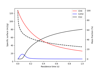
class bloc.reactors.CarbonBlackIdealGasMoleReactor(*args, **kwargs)#

Bases: cantera.ExtensibleIdealGasMoleReactor

IdealGasMoleReactor with additional features for carbon quality calculations.

This class extends the cantera.IdealGasMoleReactor class to include additional features for carbon quality calculations. The class is intended to be used in Reactor Networks.

Examples

residence_time#: Residence time in (s). Residence time must be set by the user during simulation.

after_initialize(t0)#

guess_specific_surface(Model=KirkOthmer2004SurfaceArea)#

Evaluate the specific surface of the carbon based on temperature and residence time.

Note

The residence time must be calculated before calling this method; for instance with:

reactor.residence_time = reactor.volume / flow_rate

Or:

for t in logspace(0.001, 1, 50):  # s
    sim.advance(t)
    reactor.residence_time = t

Parameters:: Model (class) – Surface area model to use. Default is KirkOthmer2004SurfaceArea.

Examples

class bloc.reactors.CarbonBlackIdealGasReactor(*args, **kwargs)#

Bases: cantera.ExtensibleIdealGasReactor

IdealGasReactor with additional features for carbon quality calculations.

This class extends the cantera.IdealGasReactor class to include additional features for carbon quality calculations. The class is intended to be used in Reactor Networks.

Examples

residence_time#: Residence time in (s). Residence time must be set by the user during simulation.

after_initialize(t0)#

guess_specific_surface(Model=KirkOthmer2004SurfaceArea)#

Evaluate the specific surface of the carbon based on temperature and residence time.

Note

The residence time must be calculated before calling this method; for instance with:

reactor.residence_time = reactor.volume / volumetric_flow_rate

Or:

for t in logspace(0.001, 1, 50):  # s
    sim.advance(t)
    reactor.residence_time = t

Parameters:: Model (class) – Surface area model to use. Default is KirkOthmer2004SurfaceArea.

Examples

bloc.reactors.is_psr_mixing_kind(kind)#

Return True when kind is a registered STONE kind for any PSR-family mixer.

“Any PSR-family mixer” means PSR or a subclass — e.g. the SPRING ContinuousMixingReactor (TMR) and InstantaneousMixingReactor kinds. Resolved via Boulder’s schema registry (reactor_class passed to register_reactor_builder), the same mechanism is_torch_reactor_kind() uses — so a new well-mixed-reactor subclass is recognized automatically; no hardcoded kind-name or node-id list to maintain.

class bloc.reactors.ContinuousMixingReactor(gas, *args, **kwargs)#

Bases: bloc.reactors.stirred.PSR

Industrial Torch Mixing Reactor (TMR) / multi-inlet well-mixed vessel.

A perfectly stirred reactor (see PSR) used to model the turbulent mixing of two or more streams at the outlet of a plasma torch.

STONE kind: ContinuousMixingReactor. Node id in SPRING YAML: tmr (the TMR in SPRING A3/A4).

Use this kind for any well-mixed stage where axial gradients are negligible. Assume Da_mix ≫ 1: mixing inside the vessel is faster than chemistry so the CSTR approximation holds.

Network topology#

Stage YAML: OPEN — multi-inlet MFCs, outlet PC/MFC; solved with ReactorNet and advance_to_steady_state (default).

Inner physics: OPEN CSTR. t_res_s sizes volume via Bloc post-build (_post_build_design_volumes(), V = τ·ṁ/ρ); it is the design residence time, not the stage advance_time.

See also

PSR: underlying numerical engine.
InstantaneousMixingReactor: closed-parcel alternative when inlet streams are pre-mixed algebraically before chemistry.

NETWORK_CLASS = None#

before_update_state(y)#

Inject a pending initial state into CVODE’s y before the first eval.

class bloc.reactors.InstantaneousMixing(gas, *args, **kwargs)#

Bases: bloc.reactors.stirred.PSR

Engine: instantaneous HP mix of two inlet streams + closed-τ chemistry.

Step 1 — inlet streams are combined with constant-HP algebraic mixing (mix_two_streams()), reproducing the Da_mix ≫ 1 assumption (turbulent mixing much faster than chemistry).

Step 2 — a closed constant-pressure parcel integrates the ODE from t = 0 to t = t_res_s with no inlet/outlet mass exchange.

This formalises the legacy pattern:

gas_mixed = mix_two_streams(gas_1, qm_1, gas_2, qm_2)
PSR_simu = solve_adiabatic_reactor(qm_total, 0, t_res_s, ...)

_states#

Residence-time profile recorded by solve_premixed().

Type:: ct.SolutionArray or None

NETWORK_CLASS: ClassVar[type | None] = None#

solve_premixed(gas_1, qm_1, gas_2, qm_2, t_res_s, *, verbose=True)#

HP-mix two inlet streams then integrate closed chemistry for t_res_s.

Parameters:

gas_1 – Cantera Solution objects for the two inlet streams (same or different mechanisms; both must be on the stage mechanism before calling — species mapping is the caller’s responsibility).
gas_2 – Cantera Solution objects for the two inlet streams (same or different mechanisms; both must be on the stage mechanism before calling — species mapping is the caller’s responsibility).
qm_1 – Mass flow rates [kg/s] of each stream.
qm_2 – Mass flow rates [kg/s] of each stream.
t_res_s – Chemical residence time [s]; CVODE integrates 0 → t_res_s on a closed parcel (no MFC flux during integration).
verbose – Print outlet state summary.

Returns:

dict with keys ````”gas”```` (Solution) and :py:class:``”states”:py:class:``
(:class:`~cantera.SolutionArray with extra column t [s]).`

before_update_state(y)#

Inject a pending initial state into CVODE’s y before the first eval.

class bloc.reactors.InstantaneousMixingNet(reactors, meta=None)#

Bases: cantera.ReactorNet

ReactorNet subclass for instantaneous-mix + closed-τ chemistry.

Mirrors TorchInstantaneousHeatingNet: the stage network holds no live ODE reactors. advance() only validates that _post_build_design_volumes() has pre-computed the outlet profile.

Parameters:

reactors – Stage reactor list. Must contain exactly one InstantaneousMixing instance.
meta (dict, optional) – Parameters from the STONE builder, enriched by _post_build_design_volumes(): t_res_s, mass_flow_rate.

role: ClassVar[str] = 'PSR'#

advance_to_steady_state()#: Validate precomputed outlet and delegate.

solve_steady()#: Delegate steady solve to advance_to_steady_state().

advance(time)#

Validate precomputed outlet profile from post-build.

Parameters:: time – Nominal advance time [s]; unused, kept for API compatibility.

property states: cantera.SolutionArray | None#: Closed-τ residence-time profile (satisfies CustomStageNetwork).

property scalars: Dict[str, Any]#: Build parameters and outlet-state scalars.

class bloc.reactors.InstantaneousMixingReactor(gas, *args, **kwargs)#

Bases: InstantaneousMixing

Industrial model: instantaneous mix + closed chemical residence time.

Two inlet streams (e.g. torch primary + secondary injection) are combined with constant-HP algebraic mixing (mix_two_streams()), then chemistry runs for t_res_s in a closed well-mixed parcel.

STONE kind: InstantaneousMixingReactor.

Use when Da_mix ≫ 1 (turbulent mixing time ≪ chemical timescale) and the workflow is a one-shot feedforward chain (not a continuously-fed vessel). For a continuously-fed open CSTR, use ContinuousMixingReactor instead.

Network topology#

Stage YAML: OPEN — two inlet MFCs (source reservoirs or upstream reactor outlets), outlet MFC/PressureController for downstream handoff.

Inner physics: CLOSED parcel. _post_build_design_volumes() gathers both inlet states, calls solve_premixed(), and writes back to reactor.phase + syncState(). No live ODE in the stage ReactorNet.

See also

ContinuousMixingReactor: open CSTR alternative (continuous feed/discharge).
mix_two_streams: algebraic HP mixer used in step 1.

NETWORK_CLASS: ClassVar[type | None] = None#

solve_premixed(gas_1, qm_1, gas_2, qm_2, t_res_s, *, verbose=True)#

HP-mix two inlet streams then integrate closed chemistry for t_res_s.

Parameters:

gas_1 – Cantera Solution objects for the two inlet streams (same or different mechanisms; both must be on the stage mechanism before calling — species mapping is the caller’s responsibility).
gas_2 – Cantera Solution objects for the two inlet streams (same or different mechanisms; both must be on the stage mechanism before calling — species mapping is the caller’s responsibility).
qm_1 – Mass flow rates [kg/s] of each stream.
qm_2 – Mass flow rates [kg/s] of each stream.
t_res_s – Chemical residence time [s]; CVODE integrates 0 → t_res_s on a closed parcel (no MFC flux during integration).
verbose – Print outlet state summary.

Returns:

dict with keys ````”gas”```` (Solution) and :py:class:``”states”:py:class:``
(:class:`~cantera.SolutionArray with extra column t [s]).`

before_update_state(y)#

Inject a pending initial state into CVODE’s y before the first eval.

class bloc.reactors.PlasmaTorchInstantaneousHeating(gas, *args, **kwargs)#

Bases: TorchInstantaneousHeating

Industrial Plasma Torch model — instantaneous-heating variant.

Instantaneous enthalpy jump (plasma power input at eta * P_torch) followed by adiabatic constant-pressure kinetics for t_res_s (see TorchInstantaneousHeating).

STONE kind: PlasmaTorchInstantaneousHeating.

The InstantaneousHeating suffix distinguishes this model from future plasma-torch implementations that may use a different heating model (e.g., arc-discharge, spatially-resolved, or multi-temperature).

Use this kind for all plasma torch stages where the heating is quasi-instantaneous compared to the chemical relaxation time.

See also

TorchInstantaneousHeating: underlying physics class.

NETWORK_CLASS: ClassVar[type | None] = None#

property SEI_MJ_kg: float | None#

Specific Energy Input [MJ/kg] from _meta (electrical input / feed).

Available on every torch once _post_build_design_volumes() has populated electric_power_kW and mass_flow_rate on _meta.

property SEO_MJ_kg: float | None#: Specific Energy Output [MJ/kg] from _meta (thermal power to gas / feed).

solve_adiabatic(mdot, power_kW, t_res_s, verbose=True)#

Solve adiabatic kinetics using this reactor’s current inlet state.

Adds torch power as an enthalpy jump and integrates one adiabatic pass for t_res_s using a fresh type(self)(gas, clone=False) carrier.

class bloc.reactors.TorchInstantaneousHeating(gas, *args, **kwargs)#

Bases: cantera.IdealGasConstPressureMoleReactor

Torch physics engine with instantaneous enthalpy jump (plasma / simplified).

Boulder’s build_sub_network detects NETWORK_CLASS and instantiates TorchInstantaneousHeatingNet for the torch stage. That class uses the same physics as the legacy simulation_non_isothermal_reactors path: instantaneous enthalpy addition (gas.HP += Q/mdot) followed by adiabatic kinetics for t_res_s.

_meta#

Torch parameters populated by _build_torch_instantaneous() and enriched by _post_build_design_volumes().

Type:: dict

_states#

Residence-time profile written by solve_adiabatic() (extra t [s]).

Type:: ct.SolutionArray or None

See also

boulder.cantera_converter

NETWORK_CLASS: ClassVar[type | None]#

property SEI_MJ_kg: float | None#

Specific Energy Input [MJ/kg] from _meta (electrical input / feed).

Available on every torch once _post_build_design_volumes() has populated electric_power_kW and mass_flow_rate on _meta.

property SEO_MJ_kg: float | None#: Specific Energy Output [MJ/kg] from _meta (thermal power to gas / feed).

solve_adiabatic(mdot, power_kW, t_res_s, verbose=True)#

Solve adiabatic kinetics using this reactor’s current inlet state.

Adds torch power as an enthalpy jump and integrates one adiabatic pass for t_res_s using a fresh type(self)(gas, clone=False) carrier.

class bloc.reactors.TorchInstantaneousHeatingNet(reactors, meta=None)#

Bases: cantera.ReactorNet

ReactorNet subclass implementing torch adiabatic integration.

Mirrors the PFRHomogeneousShellNet pattern: overrides advance() so the torch stage runs the same physics as the legacy simulation_non_isothermal_reactors path — instantaneous enthalpy addition followed by adiabatic kinetics for t_res_s.

Parameters:

reactors – List of reactors for this stage. Must contain exactly one TorchInstantaneousHeating.
meta (dict, optional) – Parameters injected by _build_torch_instantaneous() and enriched by _post_build_design_volumes(): effective_power_kW, mass_flow_rate, t_res_s, mechanism.

role: ClassVar[str] = 'torch'#

advance_to_steady_state()#

Validate that precomputed torch outlet data is available.

This stage does not integrate dynamics here; the outlet profile is precomputed in _post_build_design_volumes().

solve_steady()#

Delegate steady solve to advance_to_steady_state().

Base ReactorNet would run on an empty reactor list and raise.

advance(time)#

Validate and expose the precomputed torch outlet.

_post_build_design_volumes() pre-computes a torch outlet profile and stores _states before this TorchInstantaneousHeatingNet is instantiated. Downstream extraction reads torch.phase after solve_adiabatic() writeback.

Parameters:: time – Nominal advance time [s], unused and kept for API compatibility.

property states: cantera.SolutionArray | None#: Adiabatic post-enthalpy profile (satisfies CustomStageNetwork).

property scalars: Dict[str, Any]#: Torch build parameters and outlet-state physics quantities.

bloc.reactors.compute_torch_sei_mj_kg(electric_power_kW, mdot_kg_s)#

Specific Energy Input [MJ/kg] = electrical input per kg of feed.

SEI = electric_power_kW·1e3 / mdot / 1e6. Returns None when mdot_kg_s is not positive.

bloc.reactors.compute_torch_seo_mj_kg(effective_power_kW, mdot_kg_s)#

Specific Energy Output [MJ/kg] = thermal power to gas per kg of feed.

SEO = effective_power_kW·1e3 / mdot / 1e6 where effective_power_kW = electric_power_kW × torch_eff × gen_eff. Matches the SEO_torch KPI in bloc.reporting.spring_kpi. Returns None when mdot_kg_s is not positive.

bloc.reactors.is_torch_reactor_kind(kind)#

Return True when kind is a registered STONE kind for any torch.

“Any torch” means TorchInstantaneousHeating or a subclass — the base engine, PlasmaTorchInstantaneousHeating, and any supplier catalog model built on it (e.g. PBR100PlasmaTorch). Resolved via Boulder’s schema registry (reactor_class passed to register_reactor_builder), the same mechanism boulder.schema_registry.is_const_pressure_kind uses — so a new torch subclass is recognized automatically; no hardcoded kind-name list to maintain.

class bloc.reactors.PFRWallProfileNet(reactors, meta=None, *, wall_T_fn=None, total_length=None, n_points=200, rtol=0.0001, atol=1e-12)#

Stage network driving a TubeFurnace through a prescribed wall profile.

Replaces the legacy LagrangianPFRReactor + LagrangianPFRNetwork + DesignTubeFurnaceNet trio with a single driver built on the unified PFRWallProfile engine and the shared march_lagrangian_parcel() marcher.

Physics#

A closed Lagrangian gas parcel is marched from inlet to outlet. At each spatial checkpoint the wall temperature T_wall(x) and the entry-length position x_position = max(x - heating_start, 0) are pushed onto the carrier; the after_eval() hook then injects forced-convection + grey-gas-radiation flux into the energy ODE.

Numerics#

Unlike the retired adaptive net.step loop, this driver uses the fixed-checkpoint net.advance march (n_points default 200), which yields a uniform spatial grid and reproduces the experimentally-validated (Mei 2019) profiles within < 1 %. Spatial resolution is controlled by n_points alone; inner CVODE step size is left to the integrator.

The public surface is duck-typed to Boulder’s CustomStageNetwork (time, states, scalars, advance, advance_to_steady_state) and exposes the tube-furnace diagnostics (E_conv, E_rad, n_steps, h_conv_avg, Fo_D_min and the recorded *_arr profiles) consumed by compute_tube_furnace_kpis(), report_details and yaml_utils.

param reactors:: Iterable containing exactly one TubeFurnace (PFRWallProfile) reactor.
param meta:: Geometry / wall-profile parameters produced by _build_design_tube_furnace() (total_length, T_wall_K, T_ambient_K, entry_leg, exit_leg, entry_zone, plateau_zone, T_wall_profile, diameter, kappa_grey).
type meta:: dict, optional

NETWORK_DIAGRAM_NOTE: str = 'Node temperatures in this diagram reflect the outlet gas state of the Lagrangian simulation...#

reactors#

E_conv: float = 0.0#

E_rad: float = 0.0#

n_steps: int = 0#

h_conv_avg: float#

Fo_D_min: float#

x_arr: numpy.ndarray | None = None#

t_arr: numpy.ndarray | None = None#

T_wall_arr: numpy.ndarray | None = None#

T_gas_arr: numpy.ndarray | None = None#

Y_Cs_arr: numpy.ndarray | None = None#

X_arr: numpy.ndarray | None = None#

species_names: list[str] | None = None#

Fo_D_arr: numpy.ndarray | None = None#

h_conv_arr: numpy.ndarray | None = None#

alpha_arr: numpy.ndarray | None = None#

u_arr: numpy.ndarray | None = None#

k_arr: numpy.ndarray | None = None#

Re_arr: numpy.ndarray | None = None#

Pr_arr: numpy.ndarray | None = None#

property reactor: bloc.reactors.plug_flow.PFRWallProfile#: The single PFRWallProfile/TubeFurnace reactor (used by plot helpers).

property mass_flow_rate: float#: Mass flow rate [kg/s] of the driven reactor.

property network#: Self-reference kept for backward compatibility with diagnostics readers.

property time: float#: Residence time [s] of the Lagrangian march (0 before advance).

property preconditioner#: Preconditioner is managed inside march_lagrangian_parcel; exposed for symmetry.

solve_steady()#: Delegate to advance_to_steady_state() for Boulder solve_steady.

advance(t=1.0)#: Advance to t; for a Lagrangian tube this runs to the outlet.

advance_to_steady_state()#

Run the fixed-checkpoint parcel march from inlet to outlet.

The full axial cantera.SolutionArray is attached to the reactor as _states (consumed by Boulder’s stage-state collector and spatial_series_fn). Idempotent: a second call is a no-op.

property states: cantera.SolutionArray | None#: Axial Lagrangian profile (satisfies Boulder’s stage-state collector).

property scalars: Dict[str, Any]#: Tube-furnace scalars (wall energy budget, residence time, meta).

draw(title='Tube Furnace — Wall Temperature Profile', n_points=200)#

Return a schematic matplotlib Figure of the tube-furnace geometry.

Upper panel: colour-coded tube rectangle (cold→hot→cold). Lower panel: wall (and, post-advance, gas) temperature profile. Does not require advance() — relies only on wall_T_fn/total_length.

plot_temperature_profile(title='Temperature Profile — Tube Furnace')#

Plot gas + wall temperature vs position with a residence-time axis.

Requires advance_to_steady_state() to have been called.

plot_species_profiles(species=None, title='Species Profile — Tube Furnace')#

Plot mole-fraction profiles vs position with a residence-time axis.

Requires advance_to_steady_state() to have been called. When species is None, the six species with the highest peak mole fraction (≥ 0.1 %) are selected automatically.

class bloc.reactors.SootRadiatingTubeFurnace(gas, *args, clone=False, diameter=0.1, kappa_grey=0.0, mass_flow_rate=0.0, soot_density=1800.0, n_C_min=None, **kwargs)#

Bases: TubeFurnace

Tube furnace with soot-augmented grey-gas radiation.

Overrides the energy-balance hook so the radiative flux uses an effective absorption coefficient kappa = kappa_grey + kappa_soot evaluated from the local gas state, instead of the fixed self.kappa_grey used by the base class. kappa_grey therefore carries the clean-gas baseline.

Soot contribution uses the Planck-mean grey-gas correlation (Rodrigues):

\[\kappa_{soot} = 3.83\,\frac{C_0}{C_2}\,f_v\,T\]

where:

\(f_v = Y_{soot}\,\rho_{gas}/\rho_{soot}\) is the local soot volume fraction, with \(Y_{soot}\) the summed solid-carbon mass fraction, \(\rho_{gas}\) the gas density, and \(\rho_{soot}\) the soot particle density (soot_density, default 1800 kg/m³).
\(C_0 = 6\pi\,E(m)\) is the soot optical constant, with \(E(m) \approx 0.260\) the soot absorption function (dimensionless). Implemented as _SOOT_C0 = 6 * pi * 0.260.
\(C_2 = hc/k_B\) is the second radiation constant (Planck law), \(C_2 \approx 0.014388\) m·K. Implemented as _SOOT_C2.

The prefactor 3.83 and the \(C_0/C_2\) grouping are folded into _SOOT_KAPPA_COEFF in code.

References

Rodrigues, P. Modélisation multiphysique de flammes turbulentes suitées avec la prise en compte des transferts radiatifs et des transferts de chaleur pariétaux.

soot_density#

n_C_min = None#

after_eval(t, LHS, RHS)#: Inject wall convection + soot-augmented grey-gas radiation.

NETWORK_CLASS: ClassVar[type | None] = None#

SOLVER_MODE: ClassVar[str] = 'adaptive'#

diameter = 0.1#

kappa_grey = 0.0#

mass_flow_rate = 0.0#

T_wall_K: float | None = None#

x_position: float = 0.0#

before_update_state(y)#: Inject a pending initial state into CVODE’s y before the first eval.

heat_flux_factory(carrier)#

Return a heat-flux callable Q(t) [W/m²] for this wall model.

Override in subclasses to provide the wall heat-transfer law. Return None for an adiabatic parcel.

Parameters:: carrier – The fresh closed-carrier instance created by build_closed_carrier_net(). Subclasses may read carrier attributes (diameter, phase, _meta, …) to build the closure.

class bloc.reactors.TubeFurnace(gas, *args, clone=False, diameter=0.1, kappa_grey=0.0, mass_flow_rate=0.0, **kwargs)#

Bases: bloc.reactors.plug_flow.PFRWallProfile

Industrial Tube Furnace model.

A plug-flow reactor heated by an externally prescribed wall-temperature profile T_wall(x) using forced convection and grey-gas radiation (see PFRWallProfile).

STONE kind: TubeFurnace. For the STONE YAML schema see TubeFurnaceSchema.

Use this kind for any electrically or indirectly heated tube where the wall temperature profile is known or measured. The Carbon-Black tube furnace (Mei-2019 validation) is the canonical example.

See also

PFRWallProfile: underlying numerical engine.
RefractoryReactor: insulated thick-shell reactor (SPRING CGR).

NETWORK_CLASS: ClassVar[type | None] = None#

SOLVER_MODE: ClassVar[str] = 'adaptive'#

diameter = 0.1#

kappa_grey = 0.0#

mass_flow_rate = 0.0#

T_wall_K: float | None = None#

x_position: float = 0.0#

after_eval(t, LHS, RHS)#: Inject wall convection + radiation into the energy ODE RHS.

before_update_state(y)#: Inject a pending initial state into CVODE’s y before the first eval.

heat_flux_factory(carrier)#

Return a heat-flux callable Q(t) [W/m²] for this wall model.

Override in subclasses to provide the wall heat-transfer law. Return None for an adiabatic parcel.

Parameters:: carrier – The fresh closed-carrier instance created by build_closed_carrier_net(). Subclasses may read carrier attributes (diameter, phase, _meta, …) to build the closure.

bloc.reactors.compute_tube_furnace_kpis(sim)#

Compute tube-furnace engineering KPIs from a solved STONE Simulation.

Bridges the STONE/Boulder path to the same output key set as bloc.yaml_utils._tf_kpi_extractor() (the ctwrap path), so that run_yaml_scenarios.py and the legacy ctwrap runner produce the same Calculation Note Excel.

Looks for a PFRWallProfileNet in sim.network.networks (the stage solver mapping). All scalars are read from that network, which is populated during advance_to_steady_state.

Parameters:: sim (bloc.simulation_builder.Simulation) – Solved STONE simulation returned by bloc.simulation_builder.build_simulation_from_yaml().
Returns:: Flat scalar dict with keys matching bloc.yaml_utils.TF_OUTPUT_VARIABLE_MAP (T_outlet_C, E_conv_J, E_rad_J, P_conv_avg_W, P_rad_avg_W, SEO_MJ_kg, n_steps, h_conv_avg_W_m2_K, Fo_D_min, diameter_mm, t_res_s) plus per-species mole (X_*) and mass (Y_*) fractions. Returns an empty dict when no PFRWallProfileNet is found in sim.network.networks.
Return type:: dict

bloc.reactors#

Submodules#

Attributes#

Classes#

Functions#

Package Contents#

Physics#

Why not ct.FlowReactor?#

Physics#

Use cases#

Physics#

Use cases#

Not intended for#

Physics#

Use cases#

Physics#

Use cases#

Physics#

Use cases#

Network topology#

Not intended for#

Why not ct.IdealGasConstPressureMoleReactor?#

Network topology#

Network topology#

Physics#

Numerics#

Why not `ct.FlowReactor`?#

Why not `ct.IdealGasConstPressureMoleReactor`?#