—

Plug Flow Reactor.

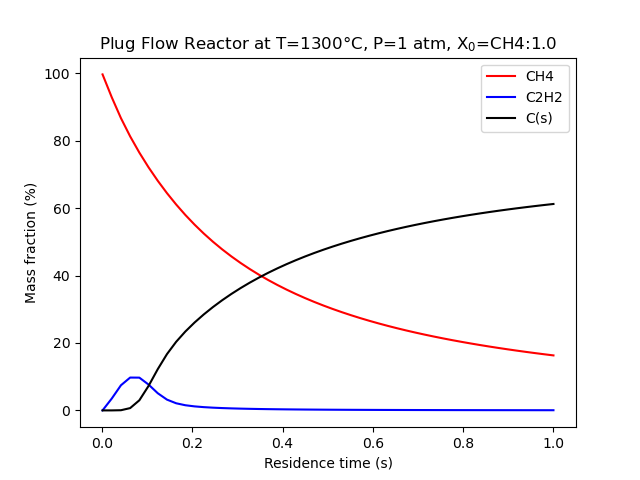
Plot Plug-Flow-Reactor (PFR) mass fractions as a function of residence time.

We use a Lagrangian approach, i.e. we track a particle in time and convert this to space, using a IdealGasConstPressureReactor reactor.

Inspired by https://cantera.org/stable/examples/python/reactors/pfr.html#method-1-lagrangian-particle-simulation

See other Plug Flow approaches in spark-cleantech-l3/bloc#13

import cantera as ct  # type: ignore
import matplotlib.pyplot as plt
import numpy as np

from bloc.utils import get_mechanism_path

mechanism = get_mechanism_path("Fincke_GRC.yaml")
composition = "CH4:1.0"

T_C = 1300  # °C
P_atm = 1  # atm

g = ct.Solution(mechanism)
g.TPX = T_C + 273.15, P_atm * ct.one_atm, composition
# Cantera units : T in K; P in Pa (converted from one_atm above)

reactor = ct.IdealGasConstPressureReactor(g, energy="off")
sim = ct.ReactorNet([reactor])

# Create a SolutionArray object to store the simulation results.
states = ct.SolutionArray(g, extra=["t"])

# Run the simulation for different residence times
for t in np.linspace(0.001, 1, 50):  # s
    sim.advance(t)
    states.append(reactor.thermo.state, t=t)

---

plt.figure()
plt.xlabel("Residence time (s)")
# Plot CH4, C2H2 and C(s) mole fractions as a function of residence time
plt.plot(states.t, states.Y[:, g.species_index("CH4")] * 100, "r-", label="CH4")
plt.plot(states.t, states.Y[:, g.species_index("C2H2")] * 100, "b-", label="C2H2")
plt.plot(
    states.t,
    states.Y[:, g.species_index("C(s)")] * 100,
    "-",
    color="black",
    label="C(s)",
)
plt.ylabel("Mass fraction (%)")
plt.legend()
plt.title(f"Plug Flow Reactor at T={T_C}°C, P={P_atm} atm, X$_0$={composition}")


plt.show()