

—
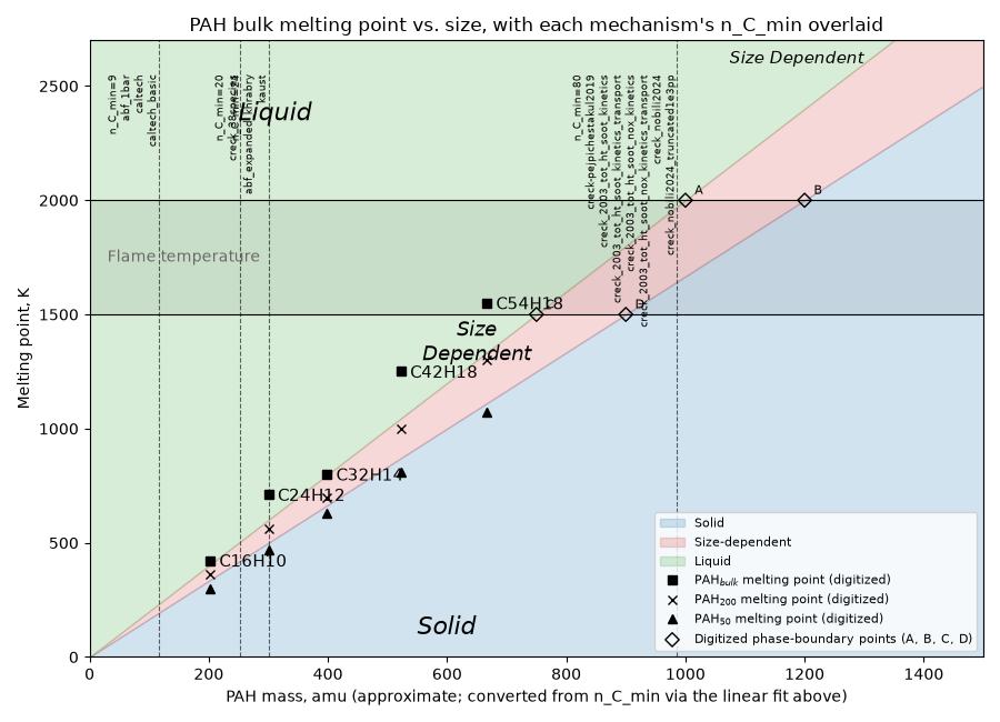
PAH size-dependent melting vs. mechanism solid-carbon thresholds.#
Every Cantera mechanism Bloc supports resolves its own solid-carbon
carbon-count threshold, n_C_min, via
resolve_n_c_min() (see
bloc.chem.solid_carbon_threshold for why the right value depends on
the mechanism). This example places each registered mechanism’s threshold
on an (approximate) PAH melting-point-vs-size phase diagram, so it’s visually
clear which mechanisms treat a given PAH size as “solid” well past the
liquid/solid transition – and which are more aggressive.
The phase diagram (Liquid / Size-dependent / Solid regions, five
labeled bulk-PAH melting points, and the two dashed boundary lines
separating the regions) is digitized by eye, approximately from Fig. 5 of
Chen et al. (2015), “Solid-liquid transitions in homogenous ovalene,
hexabenzocoronene and circumcoronene clusters: A molecular dynamics study”,
Combustion and Flame, https://doi.org/10.1016/j.combustflame.2014.07.025
(see data/literature/README.md for provenance and caveats). This is a
qualitative, order-of-magnitude comparison, not a quantitative one –
refer to the original publication for exact values.
That figure compares melting points across three cluster sizes of the same PAH molecule:
PAH50 – A cluster consisting of 50 molecules of a given peri-condensed PAH. Its melting point is treated as a lower bound for the size-dependent region, and a PAH50 cluster is about 4 nm in diameter, making it an analogue for nascent soot particles.
PAH200 – A cluster consisting of 200 molecules of a given PAH. Its size is approximately 1.5 times that of PAH50. It’s used to show how the cluster melting point changes with cluster size.
PAHbulk – The bulk (macroscopic) solid of the same PAH. Its melting point is treated as an upper bound for the size-dependent region, and it serves as an approximation for mature soot particles.
import matplotlib.pyplot as plt
import numpy as np
import pandas as pd

from bloc.chem.solid_carbon_threshold import registered_mechanisms
from bloc.paths import ROOT_FOLDER_PATH
Load the digitized bulk-PAH melting-point data and phase-boundary points#
literature_dir = ROOT_FOLDER_PATH / "data" / "literature"
pah_data = pd.read_csv(
    literature_dir / "chen2015_pah_bulk_melting_point.csv", comment="#"
)
boundary_points = pd.read_csv(
    literature_dir / "chen2015_phase_boundary_points.csv", comment="#"
)
pah_data
Map a carbon count to an approximate ring count / mass#
A linear fit through the 5 digitized (n_C, rings) / (n_C, mass) points – good enough to place a mechanism’s n_C_min on the same axes as the figure, not a physical model of PAH structure.
ring_fit = np.polyfit(pah_data["n_C"], pah_data["n_aromatic_rings"], 1)
mass_fit = np.polyfit(pah_data["n_C"], pah_data["MW_amu"], 1)


def n_c_to_mass(n_c: float) -> float:
    return float(np.polyval(mass_fit, n_c))
Group registered mechanisms by their resolved n_C_min#
Several mechanisms share the same threshold (e.g. the whole CRECK sectional-soot family uses n_C_min=80) – group them so the plot shows one line per distinct threshold instead of a dozen overlapping ones. Mechanisms with n_c_min=None (no PAH continuum, e.g. Fincke_GRC: only named C(s)/C(soot) ever count as solid) have no carbon-count threshold to place on this axis at all – listed separately below instead.
by_n_c_min: dict[int, list[str]] = {}
species_names_only: list[str] = []
for basename, result in sorted(registered_mechanisms().items()):
    if result.n_c_min is None:
        species_names_only.append(basename)
        continue
    by_n_c_min.setdefault(result.n_c_min, []).append(basename)

print("Mechanisms with no carbon-count threshold (named species only):")
for basename in species_names_only:
    result = registered_mechanisms()[basename]
    print(f"  {basename}: solid species = {result.solid_species_names}")
Mechanisms with no carbon-count threshold (named species only):
  fincke_grc: solid species = ('C(s)', 'C(soot)')
  fincke_grc_w_ar&ions: solid species = ('C(s)', 'C(soot)')
  fincke_sandia: solid species = ('C(s)', 'C(soot)')
  holmen1995_with_nucleation: solid species = ('C(s)',)
  kassel_fridman: solid species = ('C(s)',)
  kassel_plenesys: solid species = ('C(s)',)
Plot#
fig, ax = plt.subplots(figsize=(9, 6.5))

# Phase-diagram boundaries (Liquid <-> Size-dependent, Size-dependent <->
# Solid): each fit through its two digitized anchor points (A+C, B+D --
# see data/literature/README.md). A straight-line fit, not a physical model.
mass_range = np.linspace(0, 1500, 200)


def _boundary_fit(name: str):
    pts = boundary_points[boundary_points["boundary"] == name]
    slope, intercept = np.polyfit(pts["MW_amu"], pts["melting_point_K"], 1)
    return slope * mass_range + intercept


upper_boundary = _boundary_fit("liquid_size_dependent")  # Size-dependent <-> Liquid
lower_boundary = _boundary_fit("size_dependent_solid")  # Solid <-> Size-dependent

ax.fill_between(
    mass_range, 0, lower_boundary, color="tab:blue", alpha=0.20, label="Solid"
)
ax.fill_between(
    mass_range,
    lower_boundary,
    upper_boundary,
    color="tab:red",
    alpha=0.18,
    label="Size-dependent",
)
ax.fill_between(
    mass_range, upper_boundary, 2700, color="tab:green", alpha=0.18, label="Liquid"
)

# "Flame temperature" band, as in the source figure: a shaded horizontal
# strip between the two reference temperatures the boundary points (A/B and
# C/D) were digitized at (2000 K and 1500 K), with solid horizontal lines at
# each edge and a label.
ax.axhspan(1500, 2000, color="gray", alpha=0.15, zorder=0)
ax.axhline(2000, color="k", linewidth=0.8)
ax.axhline(1500, color="k", linewidth=0.8)
ax.text(
    30, 1750, "Flame temperature", fontsize=10, va="center", ha="left", color="dimgray"
)

# Region labels, as in the source figure (italic text inside each region,
# rather than relying on the legend alone). "Size Dependent" is labeled twice
# (center and upper-right) since that band spans the full width of the plot.
ax.text(250, 2350, "Liquid", fontsize=16, fontstyle="italic", ha="left")
ax.text(650, 1300, "Size\nDependent", fontsize=13, fontstyle="italic", ha="center")
ax.text(1300, 2600, "Size Dependent", fontsize=11, fontstyle="italic", ha="right")
ax.text(550, 100, "Solid", fontsize=16, fontstyle="italic", ha="left")

# Three cluster sizes of the same PAH, matching the source figure's own
# marker convention: squares (PAHbulk), crosses (PAH200), triangles (PAH50).
# Markers only (no connecting line) -- the digitized points aren't dense
# enough for a line between them to mean anything beyond the marker itself.
ax.plot(
    pah_data["MW_amu"],
    pah_data["melting_point_K"],
    "ks",
    label=r"PAH$_{bulk}$ melting point (digitized)",
)
ax.plot(
    pah_data["MW_amu"],
    pah_data["melting_point_K_pah200"],
    "kx",
    label=r"PAH$_{200}$ melting point (digitized)",
)
ax.plot(
    pah_data["MW_amu"],
    pah_data["melting_point_K_pah50"],
    "k^",
    label=r"PAH$_{50}$ melting point (digitized)",
)
for _, row in pah_data.iterrows():
    ax.annotate(
        row["formula"],
        (row["MW_amu"], row["melting_point_K"]),
        textcoords="offset points",
        xytext=(6, -4),
        fontsize=11,
    )

# The 4 digitized boundary-line anchor points themselves (A, B, C, D in the
# source figure), so the fitted boundaries above can be visually checked
# against the points they were fit through.
ax.scatter(
    boundary_points["MW_amu"],
    boundary_points["melting_point_K"],
    marker="D",
    facecolors="none",
    edgecolors="k",
    s=40,
    label="Digitized phase-boundary points (A, B, C, D)",
)
for _, row in boundary_points.iterrows():
    ax.annotate(
        row["label"],
        (row["MW_amu"], row["melting_point_K"]),
        textcoords="offset points",
        xytext=(6, 4),
        fontsize=8,
    )

for n_c_min, basenames in sorted(by_n_c_min.items()):
    mass = n_c_to_mass(n_c_min)
    ax.axvline(mass, color="k", linestyle="--", linewidth=0.8, alpha=0.6)
    label = f"n_C_min={n_c_min}\n" + "\n".join(basenames)
    ax.text(mass, 2550, label, rotation=90, va="top", ha="right", fontsize=6.5)

ax.set_xlim(0, 1500)
ax.set_ylim(0, 2700)
ax.set_xlabel(
    "PAH mass, amu (approximate; converted from n_C_min via the linear fit above)"
)
ax.set_ylabel("Melting point, K")
ax.set_title("PAH bulk melting point vs. size, with each mechanism's n_C_min overlaid")
ax.legend(loc="lower right", fontsize=8)
plt.tight_layout()
plt.show()
Total running time of the script: (0 minutes 0.286 seconds)